Strategic Information System: Business Cost Analysis and Regression

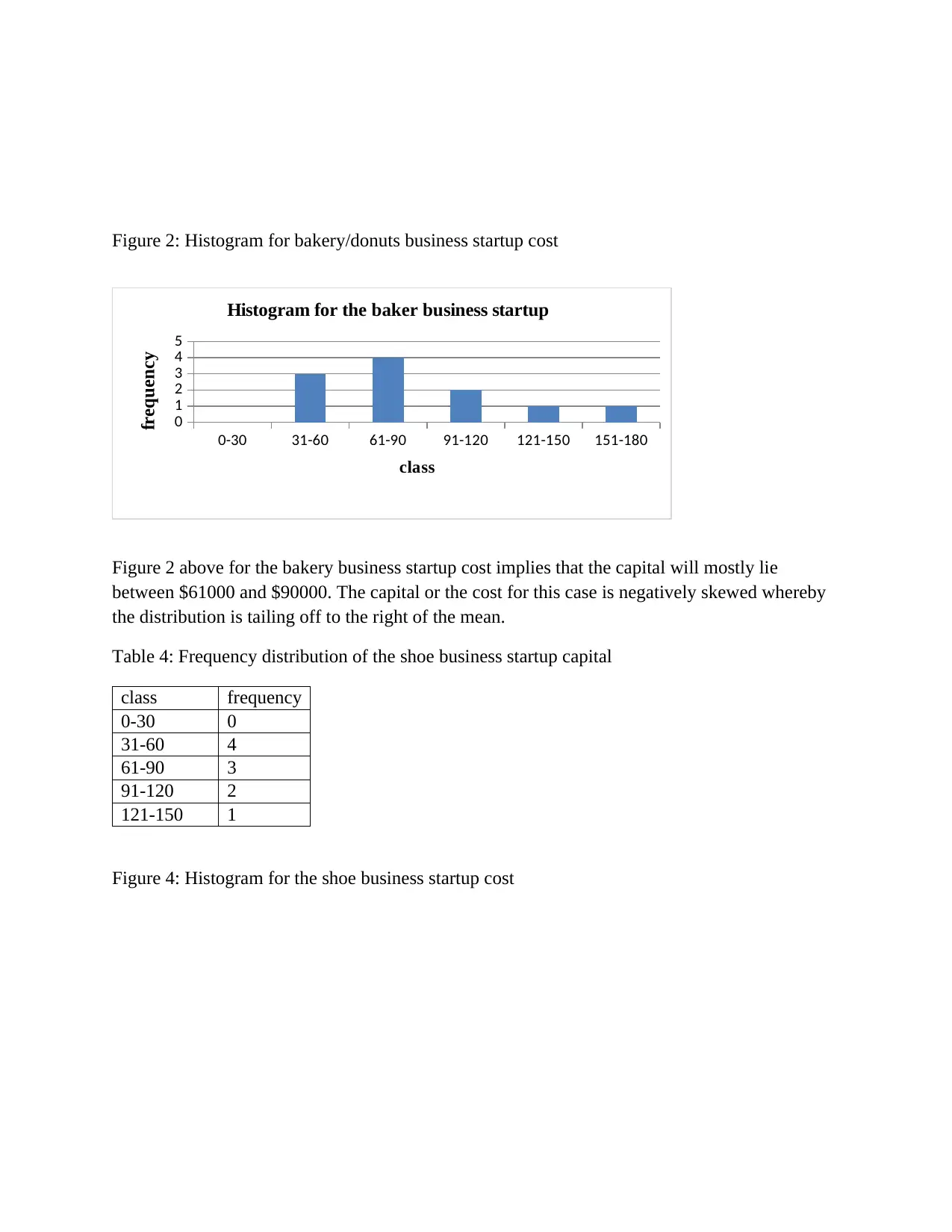
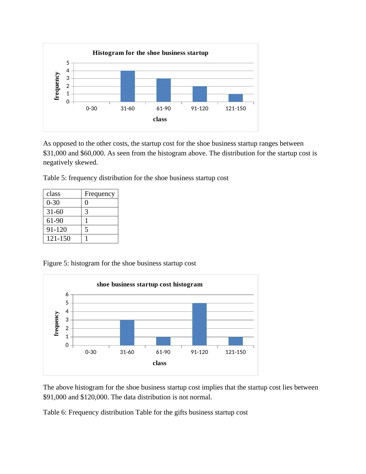
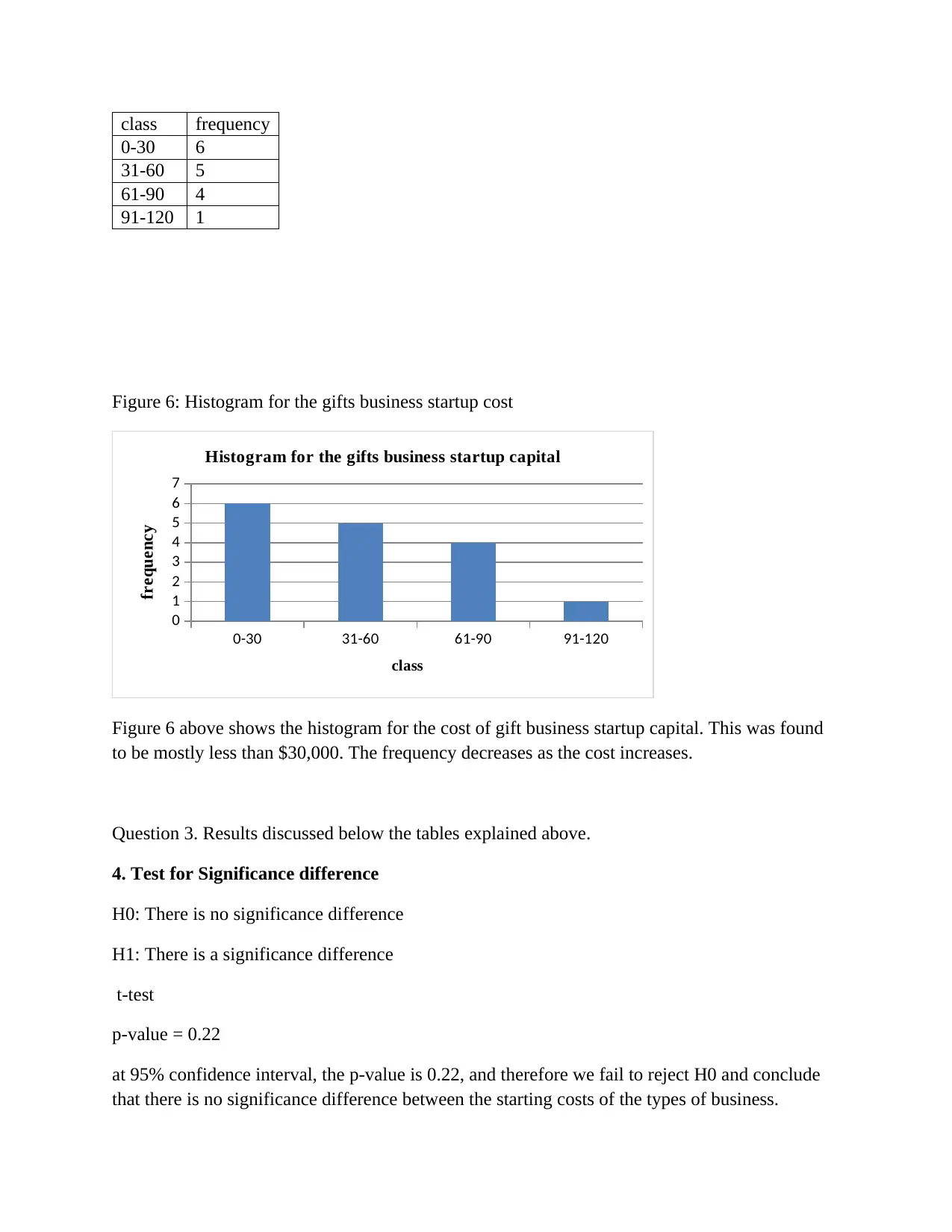
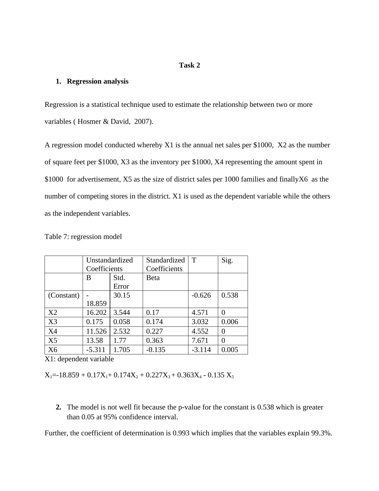
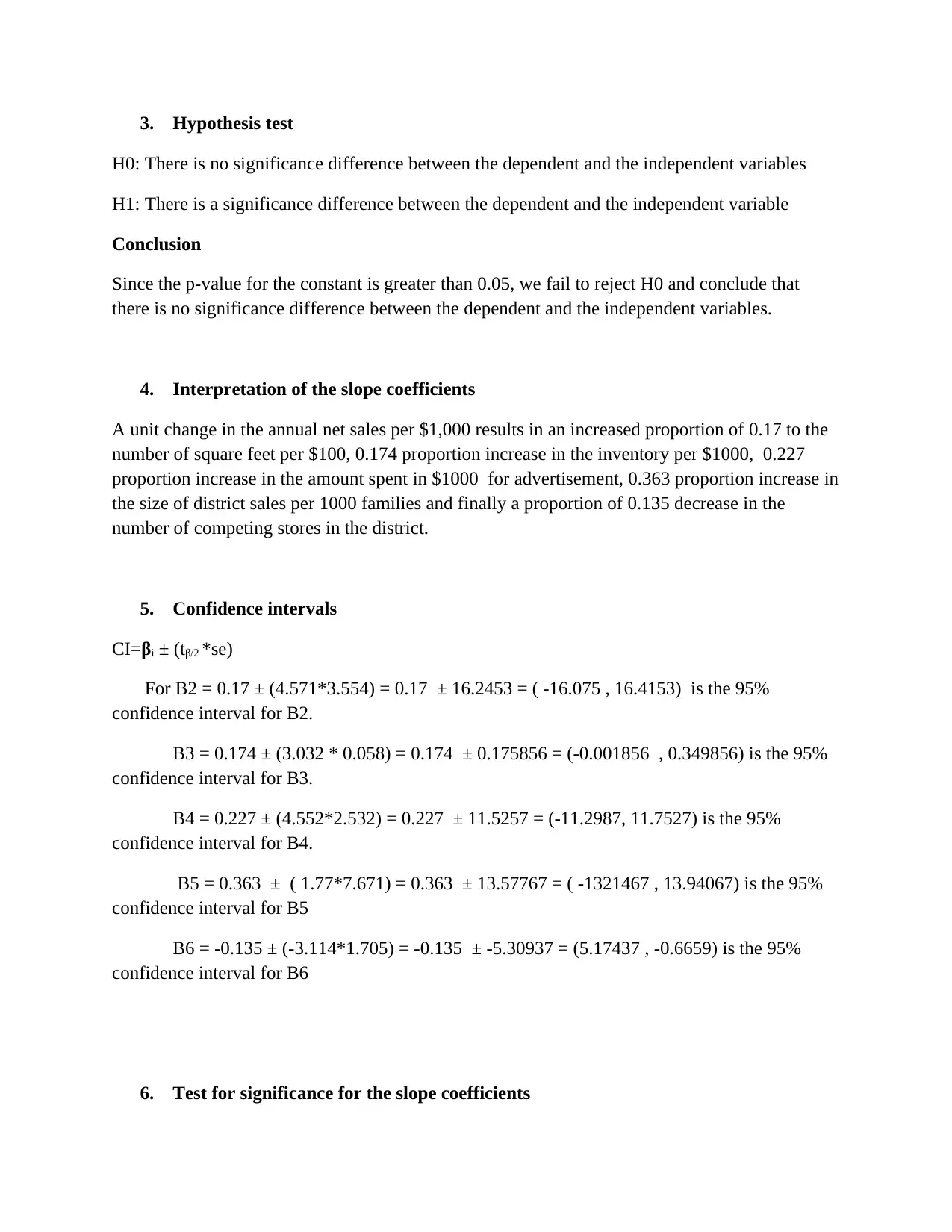
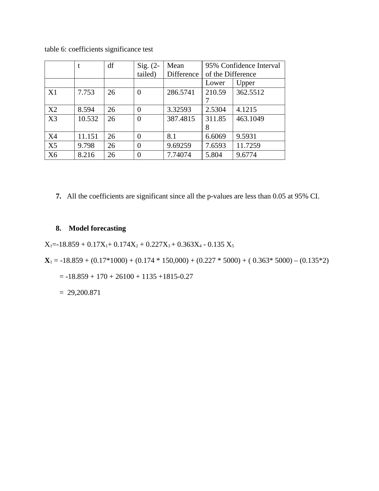
This assignment analyzes business startup costs across different business types (pizza, bakery, shoe, gift, and pet stores) using descriptive statistics, including mean, variance, standard deviation, range, and mode. It presents frequency distributions and histograms to visualize the data. The assignment also performs a t-test to determine if there's a significant difference between the startup costs of different businesses. Furthermore, it conducts a regression analysis to model the relationship between annual net sales and various factors like square footage, inventory, advertising spend, district sales size, and the number of competing stores, interpreting coefficients, confidence intervals, and testing for significance to predict future sales. Finally, it offers a model forecasting example.

Strategic Information System
Student’s Name
The Name of the Course
Instructor’s Name
Date

Task 1
Question 1
a. Mean = ∑ xi
n = 1079/13=83 the mean cost for pizza business startup is 83.
b. Mean cost for baker business startup is 1013 / 11 = 92.0909
c. the mean startup cost for shoe stores is 723 / 10 = 72.3
d. the mean startup cost for gift shop is 870 / 10 = 87
e. the mean startup cost for pet stores is 826 / 16 = 51.625
According to Jackie (2006), variance is the deviation of variable values from their mean, while
standard deviation is the deviation from the mean. Range is the difference between the highest
observation and the lowest observation. On the other hand, mode is the observation that occurs
mostly in a distribution of variables.
Variance =( Xi−x
n−1 ¿ standard deviation = √( Xi−x
n−1 ¿
Variabl
e
N Range Minimum Maximum Sum Mean Std. Deviation Variance Mode
X1 13 105 35 140 1079 83 34.135 1165.167 35
X2 11 120 40 160 1013 92.09 38.893 1512.691 N/A
X3 10 90 35 125 723 72.3 31.365 983.789 N/A
X4 10 115 35 150 870 87 35.904 1289.111 100
X5 16 90 20 110 826 51.63 27.075 733.05 30

Question 2
Table 1: Descriptive statistics for the variables
The above table shows the summary descriptive statistics where X1 the cost for pizza business
startup, X2 represents the cost for baker business startup, X3 the cost for shoe business startup,
X4 the cost for the gift shop business startup and finally X5 the cost for pet store business
startup. As seen from the table, the summary represents the respective descriptive statistics for
the range, minimum, maximum, sum, mean, standard deviation, variance and the mode for X1,
X2, X3, X4, and X5.
Frequency Distributions
Frequency distribution for the pizza cost business startup
Table 2: frequency distribution for the pizza business startup.
Class frequency
0-30 2
31-60 1
61-90 5
91-120 3
121-150 2

Figure 1: Histogram of the frequency distribution for the pizza business startup
0-30 31-60 61-90 91-120 121-150
0
1
2
3
4
5
6
histogram for the pizza business startup
class
frequency
The histogram above for the distribution of the pizza business startup cost shows that the capital
ranges mostly between $ 61,000 and $90,000. The capital is normally distributed.
Table 3: Frequency distribution for baker business startup cost
class frequency
0-30 0
31-60 3
61-90 4
91-120 2
121-150 1
151-180 1

Figure 2: Histogram for bakery/donuts business startup cost
0-30 31-60 61-90 91-120 121-150 151-180
0
1
2
3
4
5
Histogram for the baker business startup
class
frequency
Figure 2 above for the bakery business startup cost implies that the capital will mostly lie
between $61000 and $90000. The capital or the cost for this case is negatively skewed whereby
the distribution is tailing off to the right of the mean.
Table 4: Frequency distribution of the shoe business startup capital
class frequency
0-30 0
31-60 4
61-90 3
91-120 2
121-150 1
Figure 4: Histogram for the shoe business startup cost

0-30 31-60 61-90 91-120 121-150
0
1
2
3
4
5
Histogram for the shoe business startup
class
frequency
As opposed to the other costs, the startup cost for the shoe business startup ranges between
$31,000 and $60,000. As seen from the histogram above. The distribution for the startup cost is
negatively skewed.
Table 5: frequency distribution for the shoe business startup cost
class Frequency
0-30 0
31-60 3
61-90 1
91-120 5
121-150 1
Figure 5: histogram for the shoe business startup cost
0-30 31-60 61-90 91-120 121-150
0
1
2
3
4
5
6
shoe business startup cost histogram
class
frequency
The above histogram for the shoe business startup cost implies that the startup cost lies between
$91,000 and $120,000. The data distribution is not normal.
Table 6: Frequency distribution Table for the gifts business startup cost

class frequency
0-30 6
31-60 5
61-90 4
91-120 1
Figure 6: Histogram for the gifts business startup cost
0-30 31-60 61-90 91-120
0
1
2
3
4
5
6
7
Histogram for the gifts business startup capital
class
frequency
Figure 6 above shows the histogram for the cost of gift business startup capital. This was found
to be mostly less than $30,000. The frequency decreases as the cost increases.
Question 3. Results discussed below the tables explained above.
4. Test for Significance difference
H0: There is no significance difference
H1: There is a significance difference
t-test
p-value = 0.22
at 95% confidence interval, the p-value is 0.22, and therefore we fail to reject H0 and conclude
that there is no significance difference between the starting costs of the types of business.

Task 2
1. Regression analysis
Regression is a statistical technique used to estimate the relationship between two or more
variables ( Hosmer & David, 2007).
A regression model conducted whereby X1 is the annual net sales per $1000, X2 as the number
of square feet per $1000, X3 as the inventory per $1000, X4 representing the amount spent in
$1000 for advertisement, X5 as the size of district sales per 1000 families and finallyX6 as the
number of competing stores in the district. X1 is used as the dependent variable while the others
as the independent variables.
Table 7: regression model
Unstandardized
Coefficients
Standardized
Coefficients
T Sig.
B Std.
Error
Beta
(Constant) -
18.859
30.15 -0.626 0.538
X2 16.202 3.544 0.17 4.571 0
X3 0.175 0.058 0.174 3.032 0.006
X4 11.526 2.532 0.227 4.552 0
X5 13.58 1.77 0.363 7.671 0
X6 -5.311 1.705 -0.135 -3.114 0.005
X1: dependent variable
X1=-18.859 + 0.17X1+ 0.174X2 + 0.227X3 + 0.363X4 - 0.135 X5
2. The model is not well fit because the p-value for the constant is 0.538 which is greater
than 0.05 at 95% confidence interval.
Further, the coefficient of determination is 0.993 which implies that the variables explain 99.3%.

3. Hypothesis test
H0: There is no significance difference between the dependent and the independent variables
H1: There is a significance difference between the dependent and the independent variable
Conclusion
Since the p-value for the constant is greater than 0.05, we fail to reject H0 and conclude that
there is no significance difference between the dependent and the independent variables.
4. Interpretation of the slope coefficients
A unit change in the annual net sales per $1,000 results in an increased proportion of 0.17 to the
number of square feet per $100, 0.174 proportion increase in the inventory per $1000, 0.227
proportion increase in the amount spent in $1000 for advertisement, 0.363 proportion increase in
the size of district sales per 1000 families and finally a proportion of 0.135 decrease in the
number of competing stores in the district.
5. Confidence intervals
CI=βi ± (tβ/2 *se)
For B2 = 0.17 ± (4.571*3.554) = 0.17 ± 16.2453 = ( -16.075 , 16.4153) is the 95%
confidence interval for B2.
B3 = 0.174 ± (3.032 * 0.058) = 0.174 ± 0.175856 = (-0.001856 , 0.349856) is the 95%
confidence interval for B3.
B4 = 0.227 ± (4.552*2.532) = 0.227 ± 11.5257 = (-11.2987, 11.7527) is the 95%
confidence interval for B4.
B5 = 0.363 ± ( 1.77*7.671) = 0.363 ± 13.57767 = ( -1321467 , 13.94067) is the 95%
confidence interval for B5
B6 = -0.135 ± (-3.114*1.705) = -0.135 ± -5.30937 = (5.17437 , -0.6659) is the 95%
confidence interval for B6
6. Test for significance for the slope coefficients

table 6: coefficients significance test
t df Sig. (2-
tailed)
Mean
Difference
95% Confidence Interval
of the Difference
Lower Upper
X1 7.753 26 0 286.5741 210.59
7
362.5512
X2 8.594 26 0 3.32593 2.5304 4.1215
X3 10.532 26 0 387.4815 311.85
8
463.1049
X4 11.151 26 0 8.1 6.6069 9.5931
X5 9.798 26 0 9.69259 7.6593 11.7259
X6 8.216 26 0 7.74074 5.804 9.6774
7. All the coefficients are significant since all the p-values are less than 0.05 at 95% CI.
8. Model forecasting
X1=-18.859 + 0.17X1+ 0.174X2 + 0.227X3 + 0.363X4 - 0.135 X5
X1 = -18.859 + (0.17*1000) + (0.174 * 150,000) + (0.227 * 5000) + ( 0.363* 5000) – (0.135*2)
= -18.859 + 170 + 26100 + 1135 +1815-0.27
= 29,200.871

References
Hosmer, D.W. and Lemesbow, S., 2007. Goodness of fit tests for the multiple logistic regression
model. Communications in statistics-Theory and Methods, 5(14), pp.1123-1139.
Jackie, N., 2006. Introduction to Descriptive Statistics.
Owen, A.B., 2008. Empirical likelihood ratio confidence intervals for a single functional.