Experiment on Bending of Continuous Beams - Structural Mechanics L3.2
VerifiedAdded on 2023/04/23
|17
|4549
|407
Practical Assignment
AI Summary
This document presents an experiment on the bending of continuous beams, focusing on measuring bending moment distribution and comparing it with theoretical predictions. The experiment uses a 1.5m steel beam supported at three points, with strain gauges to measure strain under varying loads. The report details the apparatus, procedure, theoretical calculations using Hooke's Law and bending equations, and experimental measurements. Results are presented in tables and graphs, showing strain distribution with varying loads. The discussion analyzes the percentage of error between theoretical and experimental values, providing insights into the behavior of continuous beams under bending and highlighting the complexities of strain measurement and distribution.

BENDING OF CONTINUOUS BEAM
1
1
Paraphrase This Document
Need a fresh take? Get an instant paraphrase of this document with our AI Paraphraser

Table of Contents
1. Introduction............................................................................................................................3
2. Aims and objective.................................................................................................................3
3. Apparatus...............................................................................................................................3
4. Theory....................................................................................................................................6
5. Procedure................................................................................................................................8
6. Theoretical calculation...........................................................................................................8
7. Experimental measurement and calculation...........................................................................9
8. Result....................................................................................................................................11
9. Requirements........................................................................................................................12
10. Discussion..........................................................................................................................13
11. Conclusion..........................................................................................................................15
2
1. Introduction
A beam can be defined as a structural element that resists laterally load applied on the beam's
axis. It is majorly used in building structures such as the construction of trusses, bridges and
other structure, which carry a shear load, horizontal load and vertical load. The purpose of the
study is to examine the distribution of bending moment in a beam to understand difference
between theoretical and experimental error. In order to understand broad perspective of
bending moment, a steel beam supported on three simple supports has been taken to
investigate experimental error. Apart from experimental concept, different engineering
theories have been examined to identify strain with respect to beam.
2. Aims and objective
The aim of the study is to evaluate wide concept of theoretical and practical result in context
to distribution of bending moment with respect to beam.
To examine theoretical concept of beam to explore structure of beam
To examine strain and work load graph at different gauge position
To evaluate bending moment per Kgf at different gauge location
3. Apparatus
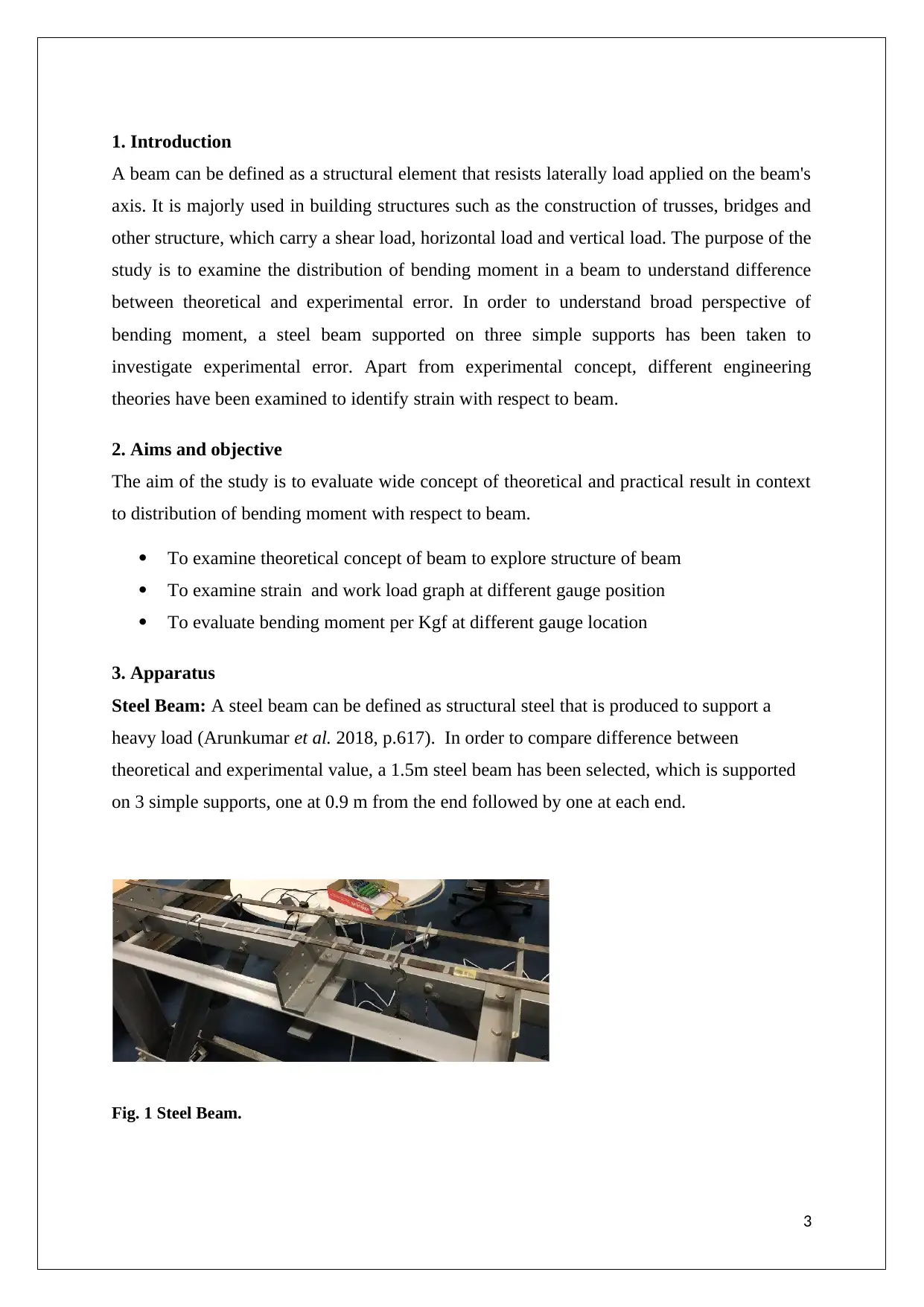
Steel Beam: A steel beam can be defined as structural steel that is produced to support a
heavy load (Arunkumar et al. 2018, p.617). In order to compare difference between
theoretical and experimental value, a 1.5m steel beam has been selected, which is supported
on 3 simple supports, one at 0.9 m from the end followed by one at each end.
Fig. 1 Steel Beam.
3
A beam can be defined as a structural element that resists laterally load applied on the beam's
axis. It is majorly used in building structures such as the construction of trusses, bridges and
other structure, which carry a shear load, horizontal load and vertical load. The purpose of the
study is to examine the distribution of bending moment in a beam to understand difference
between theoretical and experimental error. In order to understand broad perspective of
bending moment, a steel beam supported on three simple supports has been taken to
investigate experimental error. Apart from experimental concept, different engineering
theories have been examined to identify strain with respect to beam.
2. Aims and objective
The aim of the study is to evaluate wide concept of theoretical and practical result in context
to distribution of bending moment with respect to beam.
To examine theoretical concept of beam to explore structure of beam
To examine strain and work load graph at different gauge position
To evaluate bending moment per Kgf at different gauge location
3. Apparatus
Steel Beam: A steel beam can be defined as structural steel that is produced to support a
heavy load (Arunkumar et al. 2018, p.617). In order to compare difference between
theoretical and experimental value, a 1.5m steel beam has been selected, which is supported
on 3 simple supports, one at 0.9 m from the end followed by one at each end.
Fig. 1 Steel Beam.
3
⊘ This is a preview!⊘
Do you want full access?
Subscribe today to unlock all pages.
Trusted by 1+ million students worldwide

Load (W):
It is one of the important components of the experiment, which different weights have been
used between 0.5 kg to 4 kg of load so that distribution of strain on a steel beam can be
measured wisely (Classen, 2018, p.99).
Metre rule: It is used to measure the breadth of a steel beam and for that, digital meter rule
has been used to minimize the percentage of error as far as possible.
Fig. 4Metre rule
4
Paraphrase This Document
Need a fresh take? Get an instant paraphrase of this document with our AI Paraphraser

Micrometre Screw gauge
Fig. 5 Digital micrometre screw gauge & a Calliper
This is an essential apparatus for experiment, which is mostly used to measure small
dimension as compared to venirecalliper.
Strain Gauge
It is a kind of sensor and its resistance changes
with varying in applied force (Dauge and
Yosibash, 2018, p.39). The prime reason to use
this strain gauge is that it switches tension or
force into an alternation in electric resistance,
which can be measured vigilantly
Fig. 5: Strain Gauge
5

Conditioning Signal
It comprises of an eight-channel signal board, which has been selected as per National
Instruments DAQ boards.
Fig. 6 Signal Conditioning SC-2043
Application Lab of VIEW software
It is advanced and upgraded development program software, which is mostly used for
analysing data as well as control bulk application (Félix et al. 2018, p.442). The prime reason
to use this software to compare the theoretical and experiment value obtained while
experimenting so the maximum and positive outcome can be extracted.
Data Logger
It is another important apparatus in this experiment, which is mostly used to ensure that each
data can be analysis properly.
4. Theory
Hooke’s law
Hooke's law can be defined as a nature of elasticity of an object in which a small change in
the object in terms of size, area and volume are directly proportional to load or deformation
force (Metya and Balasubramaniam, 2018, p.94). This law is only applicable to the object is
under elasticity property that signifies that object can retain its original shape after removal of
the object. Mathematically, it can be represented as
F= -kx
Where, F stands for force, x stand for distance and k stand for young modulus. With the help
of this law, the elasticity limit of a steel beam can be determined, which later help in
determining value strain and load on an object (Muttoni et al. 2018, p.174). The main
6
⊘ This is a preview!⊘
Do you want full access?
Subscribe today to unlock all pages.
Trusted by 1+ million students worldwide
purpose of study is to use this law to understand change in strain at different forces both
theoretical and practical to determine experimental error positively.
Hooke’s experimental law
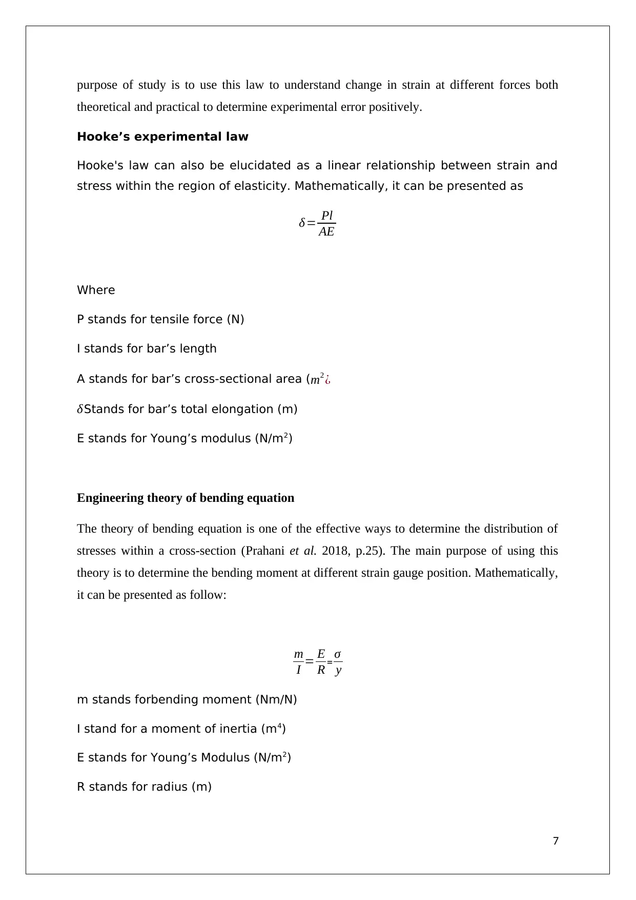
Hooke's law can also be elucidated as a linear relationship between strain and
stress within the region of elasticity. Mathematically, it can be presented as
δ = Pl
AE
Where
P stands for tensile force (N)
I stands for bar’s length
A stands for bar’s cross-sectional area (m2 ¿
δStands for bar’s total elongation (m)
E stands for Young’s modulus (N/m2)
Engineering theory of bending equation
The theory of bending equation is one of the effective ways to determine the distribution of
stresses within a cross-section (Prahani et al. 2018, p.25). The main purpose of using this
theory is to determine the bending moment at different strain gauge position. Mathematically,
it can be presented as follow:
m
I = E
R = σ
y
m stands forbending moment (Nm/N)
I stand for a moment of inertia (m4)
E stands for Young’s Modulus (N/m2)
R stands for radius (m)
7
theoretical and practical to determine experimental error positively.
Hooke’s experimental law
Hooke's law can also be elucidated as a linear relationship between strain and
stress within the region of elasticity. Mathematically, it can be presented as
δ = Pl
AE
Where
P stands for tensile force (N)
I stands for bar’s length
A stands for bar’s cross-sectional area (m2 ¿
δStands for bar’s total elongation (m)
E stands for Young’s modulus (N/m2)
Engineering theory of bending equation
The theory of bending equation is one of the effective ways to determine the distribution of
stresses within a cross-section (Prahani et al. 2018, p.25). The main purpose of using this
theory is to determine the bending moment at different strain gauge position. Mathematically,
it can be presented as follow:
m
I = E
R = σ
y
m stands forbending moment (Nm/N)
I stand for a moment of inertia (m4)
E stands for Young’s Modulus (N/m2)
R stands for radius (m)
7
Paraphrase This Document
Need a fresh take? Get an instant paraphrase of this document with our AI Paraphraser
σ Stands forstress (N/m2 ¿
y stands for the upward measured position of the beam’s mid-surface
5. Procedure
The following steps need to follow in order to perform the experiment positively
1. At first, the dimension of steel beam needs to measure including breadth b, length l
and depths with the help of micrometre screw gauge. On another hand, it needs to
ensure that the micrometrescrew gauge was wiped out including spindle so that
possible error can be reduced as far as possible for a positive result.
1. Through micrometre screw gauge, three measurements of breadth d and depth d need
to note down. The average of three value has been used while a calculation
2. With the help of Lab View 7.1, strain gauge needs to put into Zero by weight carriage
and gauge factors need to set manually (Takenaka, 2018, p.18).
3. A resistance of 210-ohm has been used to enter into gauge factor for gauges with the
execution voltage of 2.5 volts
4. In the next step, the force needs to apply with the help of varying load from 0.5 kg to
4 kg that helps in measuring the value of strain at different gauge position.
5. Base on experimental data of strain obtained by applying different load on a steel
beam, gradient value needs to measure.
6. At last, a graph needs to plot between strain against load that will help on measure
gradient or slope so that distribution of strain can be measured wisely
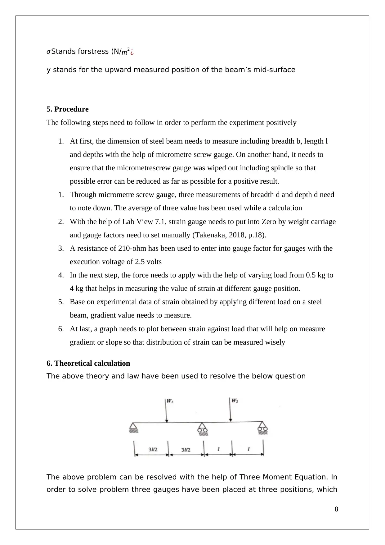
6. Theoretical calculation
The above theory and law have been used to resolve the below question
The above problem can be resolved with the help of Three Moment Equation. In
order to solve problem three gauges have been placed at three positions, which
8
y stands for the upward measured position of the beam’s mid-surface
5. Procedure
The following steps need to follow in order to perform the experiment positively
1. At first, the dimension of steel beam needs to measure including breadth b, length l
and depths with the help of micrometre screw gauge. On another hand, it needs to
ensure that the micrometrescrew gauge was wiped out including spindle so that
possible error can be reduced as far as possible for a positive result.
1. Through micrometre screw gauge, three measurements of breadth d and depth d need
to note down. The average of three value has been used while a calculation
2. With the help of Lab View 7.1, strain gauge needs to put into Zero by weight carriage
and gauge factors need to set manually (Takenaka, 2018, p.18).
3. A resistance of 210-ohm has been used to enter into gauge factor for gauges with the
execution voltage of 2.5 volts
4. In the next step, the force needs to apply with the help of varying load from 0.5 kg to
4 kg that helps in measuring the value of strain at different gauge position.
5. Base on experimental data of strain obtained by applying different load on a steel
beam, gradient value needs to measure.
6. At last, a graph needs to plot between strain against load that will help on measure
gradient or slope so that distribution of strain can be measured wisely
6. Theoretical calculation
The above theory and law have been used to resolve the below question
The above problem can be resolved with the help of Three Moment Equation. In
order to solve problem three gauges have been placed at three positions, which
8
is demonstrated below in a broad perspective (Wang et al. 2018, p.15). In addition,
bending moment at each gauge along with reaction at the supports has been
presented below:
Data are given
L =300 mm
M1 =M3 =0 [For the actual beam]
Therefore, M2 can be calculated by using Three Moment equation
M2 = 39Wl/80
V1 = 27W/80
V3 = 41W/160
Theoretically,
Bending moment/ kgf at 1 location of Gauge = V1 ×3l/2 W = 27*900/80*2 = -151.87 mm
Bending moment/ kgf at 2 location of Gauge = m2/W = 39/80*300 = 146.250 mm
Bending moment/ kgf at 3 location of Gauge = -V3*l/W = -41*300/160 = -76.87 mm
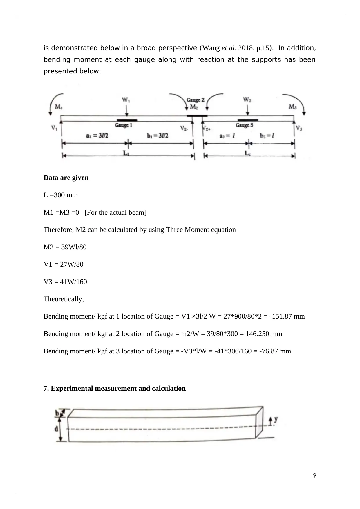
7. Experimental measurement and calculation
9
bending moment at each gauge along with reaction at the supports has been
presented below:
Data are given
L =300 mm
M1 =M3 =0 [For the actual beam]
Therefore, M2 can be calculated by using Three Moment equation
M2 = 39Wl/80
V1 = 27W/80
V3 = 41W/160
Theoretically,
Bending moment/ kgf at 1 location of Gauge = V1 ×3l/2 W = 27*900/80*2 = -151.87 mm
Bending moment/ kgf at 2 location of Gauge = m2/W = 39/80*300 = 146.250 mm
Bending moment/ kgf at 3 location of Gauge = -V3*l/W = -41*300/160 = -76.87 mm
7. Experimental measurement and calculation
9
⊘ This is a preview!⊘
Do you want full access?
Subscribe today to unlock all pages.
Trusted by 1+ million students worldwide

The above problem can be solved using above Theory and Law
According to Engineers’ theory of bending moment
m
I = E
R = σ
y
According to Hooke’s Law
δ = Pl
AE
Hence, it can be stated that
m= El
y e (1)
Given data,
E= 20,000 kgf/mm2
b= 25.38, 25.40, 25.61 mm
d= 4.92, 4.91, 4.92 mm
The above data of b and d have been measured from micrometre. In order to get an absolute
value an average of b and d have been taken into account
Average b = 25.38 + 25.40 +25.61/ 3 = 25.463 mm
Average of d = 4.92 + 4.91 + 4.92/3 = 4.91 mm
With the help of the absolute value of b and d, it is easy to determine the position of any
position.
Ytop = d/2 = 11.47/2 = 2.4583 mm
Y btm = -d/2 = 11.47/2 = -2.4583 mm
The following data related to the beam’s breadth and depth has been used to determine the
value of Inertia, which has been highlighted below:
I = bd^3/12 = 25.46*4.91^3/12 = 251.143 mm^4
10
Paraphrase This Document
Need a fresh take? Get an instant paraphrase of this document with our AI Paraphraser
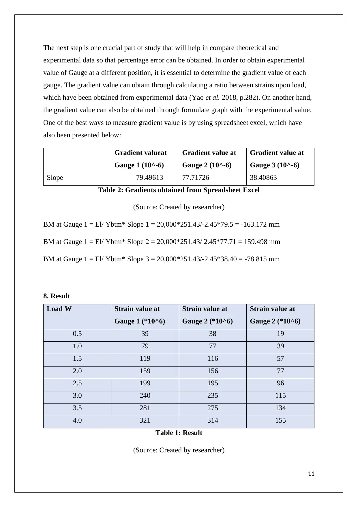
The next step is one crucial part of study that will help in compare theoretical and
experimental data so that percentage error can be obtained. In order to obtain experimental
value of Gauge at a different position, it is essential to determine the gradient value of each
gauge. The gradient value can obtain through calculating a ratio between strains upon load,
which have been obtained from experimental data (Yao et al. 2018, p.282). On another hand,
the gradient value can also be obtained through formulate graph with the experimental value.
One of the best ways to measure gradient value is by using spreadsheet excel, which have
also been presented below:
Gradient valueat
Gauge 1 (10^-6)
Gradient value at
Gauge 2 (10^-6)
Gradient value at
Gauge 3 (10^-6)
Slope 79.49613 77.71726 38.40863
Table 2: Gradients obtained from Spreadsheet Excel
(Source: Created by researcher)
BM at Gauge 1 = El/ Ybtm* Slope 1 = 20,000*251.43/-2.45*79.5 = -163.172 mm
BM at Gauge 1 = El/ Ybtm* Slope 2 = 20,000*251.43/ 2.45*77.71 = 159.498 mm
BM at Gauge 1 = El/ Ybtm* Slope 3 = 20,000*251.43/-2.45*38.40 = -78.815 mm
8. Result
Load W Strain value at
Gauge 1 (*10^6)
Strain value at
Gauge 2 (*10^6)
Strain value at
Gauge 2 (*10^6)
0.5 39 38 19
1.0 79 77 39
1.5 119 116 57
2.0 159 156 77
2.5 199 195 96
3.0 240 235 115
3.5 281 275 134
4.0 321 314 155
Table 1: Result
(Source: Created by researcher)
11
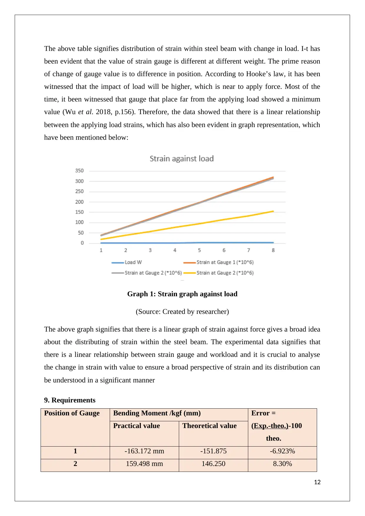
The above table signifies distribution of strain within steel beam with change in load. I-t has
been evident that the value of strain gauge is different at different weight. The prime reason
of change of gauge value is to difference in position. According to Hooke’s law, it has been
witnessed that the impact of load will be higher, which is near to apply force. Most of the
time, it been witnessed that gauge that place far from the applying load showed a minimum
value (Wu et al. 2018, p.156). Therefore, the data showed that there is a linear relationship
between the applying load strains, which has also been evident in graph representation, which
have been mentioned below:
Graph 1: Strain graph against load
(Source: Created by researcher)
The above graph signifies that there is a linear graph of strain against force gives a broad idea
about the distributing of strain within the steel beam. The experimental data signifies that
there is a linear relationship between strain gauge and workload and it is crucial to analyse
the change in strain with value to ensure a broad perspective of strain and its distribution can
be understood in a significant manner
9. Requirements
Position of Gauge Bending Moment /kgf (mm) Error =
(Exp.-theo.)-100
theo.
Practical value Theoretical value
1 -163.172 mm -151.875 -6.923%
2 159.498 mm 146.250 8.30%
12
⊘ This is a preview!⊘
Do you want full access?
Subscribe today to unlock all pages.
Trusted by 1+ million students worldwide
1 out of 17


Your All-in-One AI-Powered Toolkit for Academic Success.
+13062052269
info@desklib.com
Available 24*7 on WhatsApp / Email
![[object Object]](/_next/static/media/star-bottom.7253800d.svg)
Unlock your academic potential
Copyright © 2020–2026 A2Z Services. All Rights Reserved. Developed and managed by ZUCOL.