STT 100 T3 2018: Smartphone Usage & Hypothesis Testing in Colleges
VerifiedAdded on 2023/04/25
|11
|2245
|357
Report
AI Summary
This report investigates smartphone usage among college students, employing hypothesis testing to determine if sample data significantly differs from population statistics. The study, utilizing secondary data from a survey of 253 students, focuses on gender proportions, average monthly earnings and bills, and market share of phone types. Four hypotheses are tested, comparing sample and population means and proportions, revealing similarities in gender proportions but differences in average mobile bills. The report concludes with a discussion of potential type I and type II errors, recommending larger sample sizes for future research. This assignment provides insights into statistical analysis and hypothesis testing within the context of student behavior and technology use.

RUNNING HEADER: SMARTPHONE USAGE AMONG COLLEGE STUDENTS 1
Smartphone usage among college students
Student’s name:
Student’s ID:
Institution:
Course ID:
Smartphone usage among college students
Student’s name:
Student’s ID:
Institution:
Course ID:
Paraphrase This Document
Need a fresh take? Get an instant paraphrase of this document with our AI Paraphraser
Smartphone usage among college students 2
1. Introduction
In the contemporary society, the consumption of smartphones has been on a steep incline
(Park & Lee, 2011). As a result, this study investigates the demand of smartphones among
students in the tertiary education level. The research targets students in various colleges in
Australia. Data obtained was secondary in nature as it was obtained from an already
conducted survey at Survey Monkey. The questionnaire used for data collection contained
both open ended and close ended questions. The data collected was from 253 respondents
who represent the population of the study. A random sample of 100 participants was
selected from the data collected. The sample was selected through excel functions with an
aim of representing the whole population and ensuring that the analysis is efficient and
effective.
2. Hypothesis
The research aims to determine whether the sample selected will be significantly different to the
population. It will entail comparing whether the sample mean is equal to or not equal to the
population mean. Moreover, it will also test whether the sample proportion is equal or not equal
to the proportion of the population.
The developed hypotheses are as shown below:
H1: The male students’ proportion in the sample is equivalent to the male students’ proportion in
the population
H2: The female students’ proportion in the sample is equal to the female students’ proportion in
the population
H3: The average mobile bill of the male respondents in the population does not change when
sampled
Smartphone usage among college students 3
H4: The average mobile bill of the female respondents in the population does not change when
sampled
3. Basic Analysis
i. Proportions of male and female
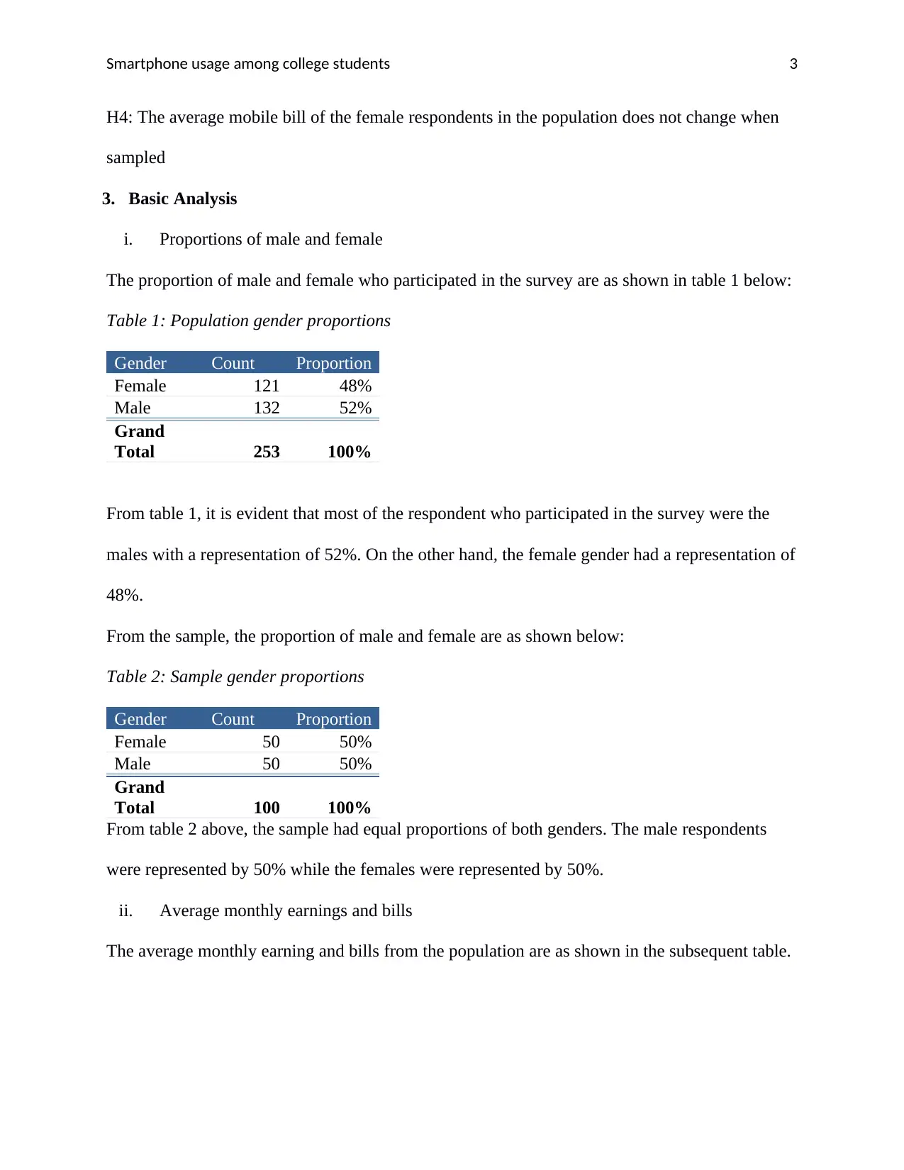
The proportion of male and female who participated in the survey are as shown in table 1 below:
Table 1: Population gender proportions
Gender Count Proportion
Female 121 48%
Male 132 52%
Grand
Total 253 100%
From table 1, it is evident that most of the respondent who participated in the survey were the
males with a representation of 52%. On the other hand, the female gender had a representation of
48%.
From the sample, the proportion of male and female are as shown below:
Table 2: Sample gender proportions
Gender Count Proportion
Female 50 50%
Male 50 50%
Grand
Total 100 100%
From table 2 above, the sample had equal proportions of both genders. The male respondents
were represented by 50% while the females were represented by 50%.
ii. Average monthly earnings and bills
The average monthly earning and bills from the population are as shown in the subsequent table.
H4: The average mobile bill of the female respondents in the population does not change when
sampled
3. Basic Analysis
i. Proportions of male and female
The proportion of male and female who participated in the survey are as shown in table 1 below:
Table 1: Population gender proportions
Gender Count Proportion
Female 121 48%
Male 132 52%
Grand
Total 253 100%
From table 1, it is evident that most of the respondent who participated in the survey were the
males with a representation of 52%. On the other hand, the female gender had a representation of
48%.
From the sample, the proportion of male and female are as shown below:
Table 2: Sample gender proportions
Gender Count Proportion
Female 50 50%
Male 50 50%
Grand
Total 100 100%
From table 2 above, the sample had equal proportions of both genders. The male respondents
were represented by 50% while the females were represented by 50%.
ii. Average monthly earnings and bills
The average monthly earning and bills from the population are as shown in the subsequent table.
⊘ This is a preview!⊘
Do you want full access?
Subscribe today to unlock all pages.
Trusted by 1+ million students worldwide
Smartphone usage among college students 4
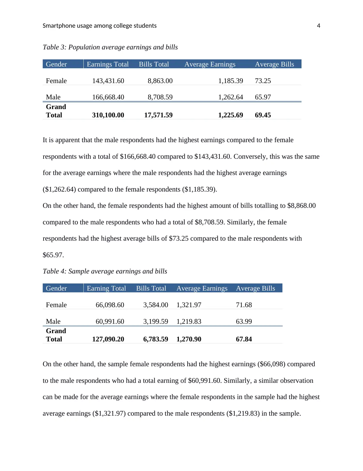
Table 3: Population average earnings and bills
Gender Earnings Total Bills Total Average Earnings Average Bills
Female 143,431.60 8,863.00 1,185.39 73.25
Male 166,668.40 8,708.59 1,262.64 65.97
Grand
Total 310,100.00 17,571.59 1,225.69 69.45
It is apparent that the male respondents had the highest earnings compared to the female
respondents with a total of $166,668.40 compared to $143,431.60. Conversely, this was the same
for the average earnings where the male respondents had the highest average earnings
($1,262.64) compared to the female respondents ($1,185.39).
On the other hand, the female respondents had the highest amount of bills totalling to $8,868.00
compared to the male respondents who had a total of $8,708.59. Similarly, the female
respondents had the highest average bills of $73.25 compared to the male respondents with
$65.97.
Table 4: Sample average earnings and bills
Gender Earning Total Bills Total Average Earnings Average Bills
Female 66,098.60 3,584.00 1,321.97 71.68
Male 60,991.60 3,199.59 1,219.83 63.99
Grand
Total 127,090.20 6,783.59 1,270.90 67.84
On the other hand, the sample female respondents had the highest earnings ($66,098) compared
to the male respondents who had a total earning of $60,991.60. Similarly, a similar observation
can be made for the average earnings where the female respondents in the sample had the highest
average earnings ($1,321.97) compared to the male respondents ($1,219.83) in the sample.
Paraphrase This Document
Need a fresh take? Get an instant paraphrase of this document with our AI Paraphraser
Smartphone usage among college students 5
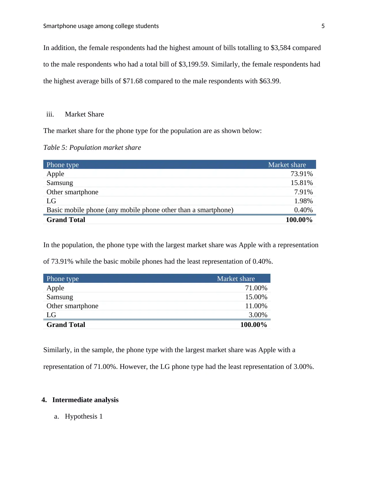
In addition, the female respondents had the highest amount of bills totalling to $3,584 compared
to the male respondents who had a total bill of $3,199.59. Similarly, the female respondents had
the highest average bills of $71.68 compared to the male respondents with $63.99.
iii. Market Share
The market share for the phone type for the population are as shown below:
Table 5: Population market share
Phone type Market share
Apple 73.91%
Samsung 15.81%
Other smartphone 7.91%
LG 1.98%
Basic mobile phone (any mobile phone other than a smartphone) 0.40%
Grand Total 100.00%
In the population, the phone type with the largest market share was Apple with a representation
of 73.91% while the basic mobile phones had the least representation of 0.40%.
Phone type Market share
Apple 71.00%
Samsung 15.00%
Other smartphone 11.00%
LG 3.00%
Grand Total 100.00%
Similarly, in the sample, the phone type with the largest market share was Apple with a
representation of 71.00%. However, the LG phone type had the least representation of 3.00%.
4. Intermediate analysis
a. Hypothesis 1
Smartphone usage among college students 6
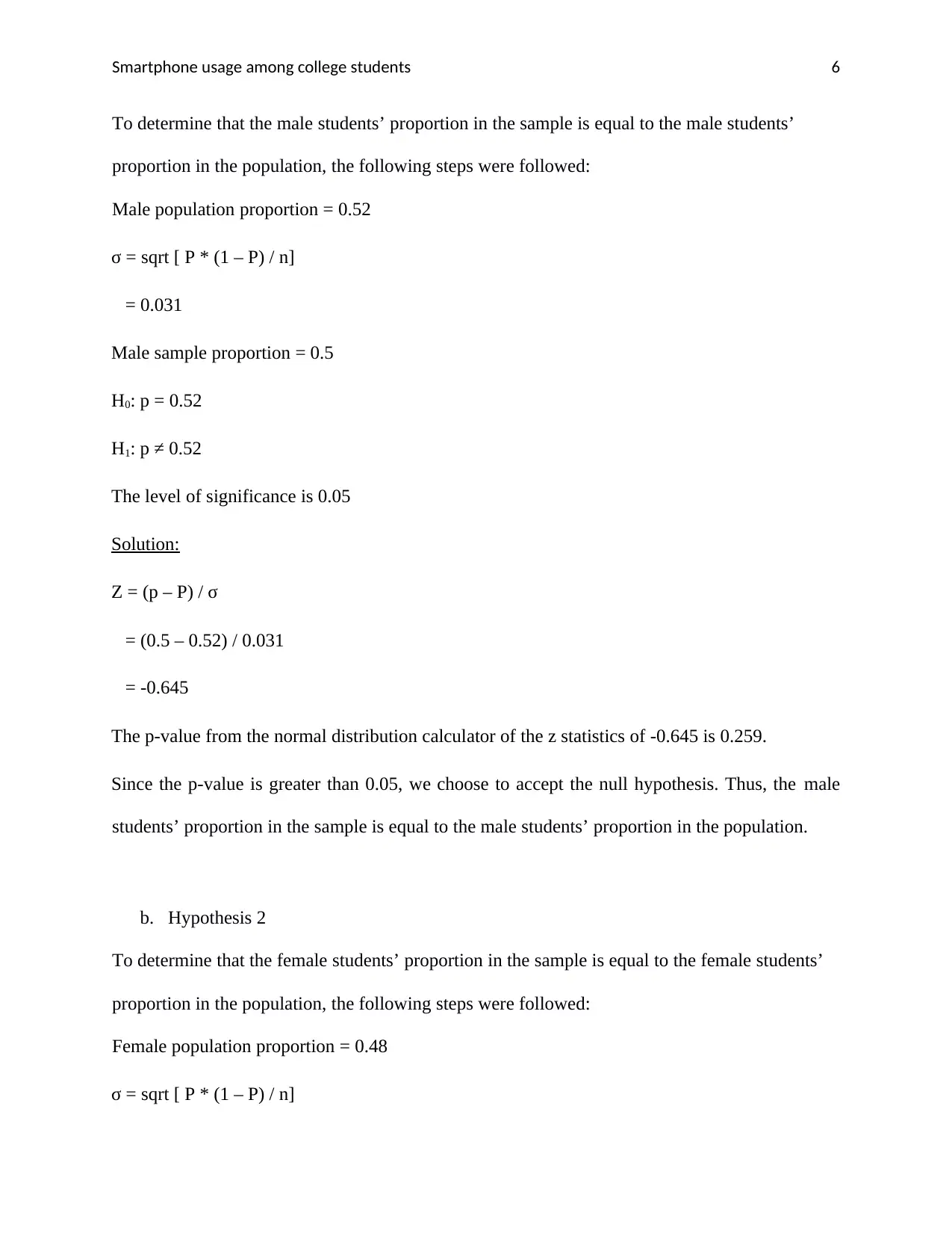
To determine that the male students’ proportion in the sample is equal to the male students’
proportion in the population, the following steps were followed:
Male population proportion = 0.52
σ = sqrt [ P * (1 – P) / n]
= 0.031
Male sample proportion = 0.5
H0: p = 0.52
H1: p ≠ 0.52
The level of significance is 0.05
Solution:
Z = (p – P) / σ
= (0.5 – 0.52) / 0.031
= -0.645
The p-value from the normal distribution calculator of the z statistics of -0.645 is 0.259.
Since the p-value is greater than 0.05, we choose to accept the null hypothesis. Thus, the male
students’ proportion in the sample is equal to the male students’ proportion in the population.
b. Hypothesis 2
To determine that the female students’ proportion in the sample is equal to the female students’
proportion in the population, the following steps were followed:
Female population proportion = 0.48
σ = sqrt [ P * (1 – P) / n]
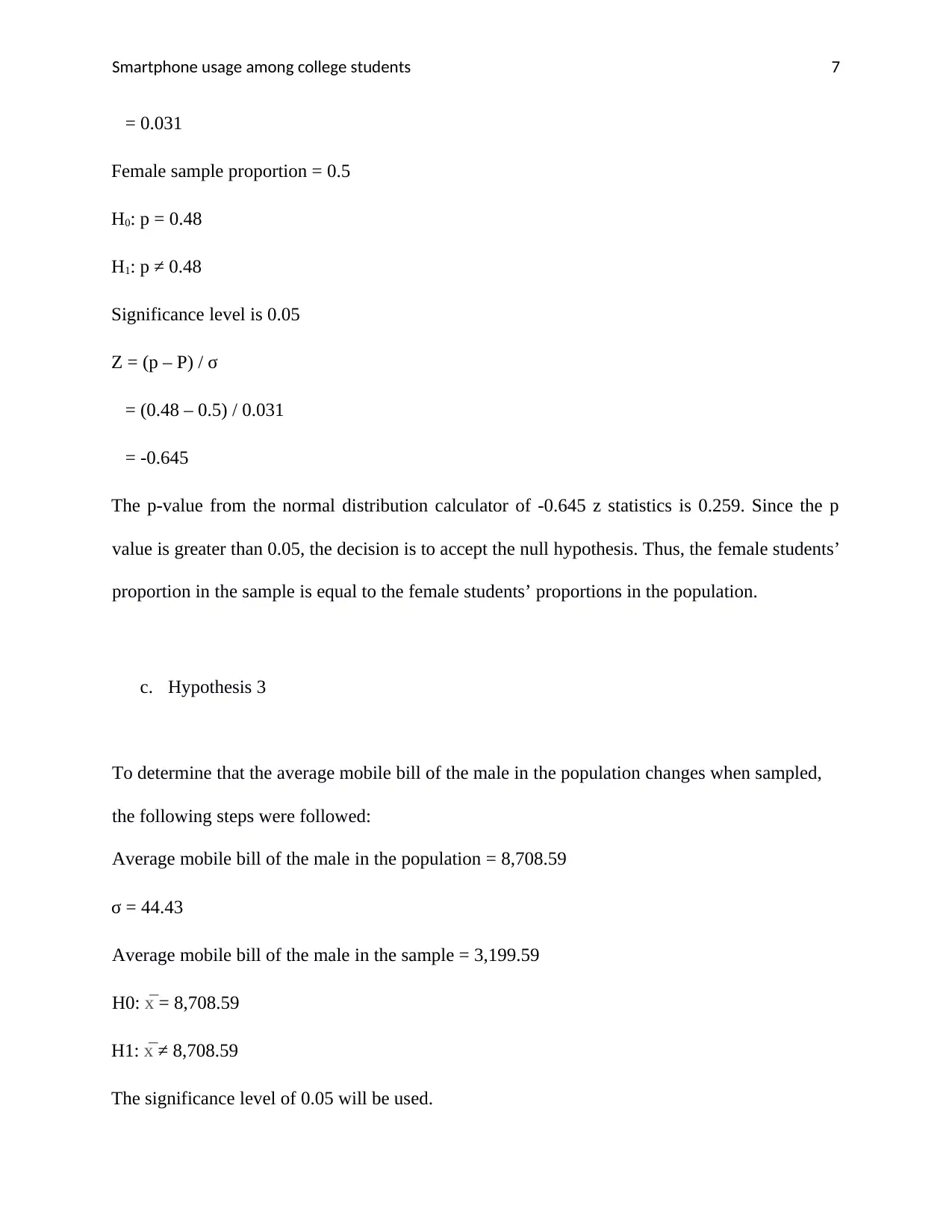
⊘ This is a preview!⊘
Do you want full access?
Subscribe today to unlock all pages.
Trusted by 1+ million students worldwide
Smartphone usage among college students 7
= 0.031
Female sample proportion = 0.5
H0: p = 0.48
H1: p ≠ 0.48
Significance level is 0.05
Z = (p – P) / σ
= (0.48 – 0.5) / 0.031
= -0.645
The p-value from the normal distribution calculator of -0.645 z statistics is 0.259. Since the p
value is greater than 0.05, the decision is to accept the null hypothesis. Thus, the female students’
proportion in the sample is equal to the female students’ proportions in the population.
c. Hypothesis 3
To determine that the average mobile bill of the male in the population changes when sampled,
the following steps were followed:
Average mobile bill of the male in the population = 8,708.59
σ = 44.43
Average mobile bill of the male in the sample = 3,199.59
H0: x̅ = 8,708.59
H1: x̅ ≠ 8,708.59
The significance level of 0.05 will be used.
Paraphrase This Document
Need a fresh take? Get an instant paraphrase of this document with our AI Paraphraser
Smartphone usage among college students 8
Z = (x̅ – μ) / (σ/sqrt(n))
= (3199.49-8708.59)/(44.43/sqrt(50))
= -876.78
The p-value of the z statistics of -876.78 is 0.00 as derived from the normal distribution
calculator.
The decision is to reject the null hypothesis since the p value is less than 0.05. Thus, the average
mobile bill of the male respondents in changes when moving from the population to the sample.
d. Hypothesis 4
To determine that the average mobile bill of the female in the population changes when sampled,
the following steps were followed:
Average mobile bill of the female in the population = 8,863.00
σ = 50.15
Average mobile bill of the female in the sample = 3,584.00
H0: x̅ = 8,863.00
H1: x̅ ≠ 8,863.00
The significance level of 0.05 will be used.
Z = (x̅ – μ) / (σ/sqrt(n))
= (3584.00-8863.00)/(50.15/sqrt(50))
= -744.33
The p-value of the z statistics of -744.33 is 0.00 derived from the normal distribution calculator.
The decision is to choose to reject the null hypothesis since the p value is less than 0.05. Thus,
Z = (x̅ – μ) / (σ/sqrt(n))
= (3199.49-8708.59)/(44.43/sqrt(50))
= -876.78
The p-value of the z statistics of -876.78 is 0.00 as derived from the normal distribution
calculator.
The decision is to reject the null hypothesis since the p value is less than 0.05. Thus, the average
mobile bill of the male respondents in changes when moving from the population to the sample.
d. Hypothesis 4
To determine that the average mobile bill of the female in the population changes when sampled,
the following steps were followed:
Average mobile bill of the female in the population = 8,863.00
σ = 50.15
Average mobile bill of the female in the sample = 3,584.00
H0: x̅ = 8,863.00
H1: x̅ ≠ 8,863.00
The significance level of 0.05 will be used.
Z = (x̅ – μ) / (σ/sqrt(n))
= (3584.00-8863.00)/(50.15/sqrt(50))
= -744.33
The p-value of the z statistics of -744.33 is 0.00 derived from the normal distribution calculator.
The decision is to choose to reject the null hypothesis since the p value is less than 0.05. Thus,
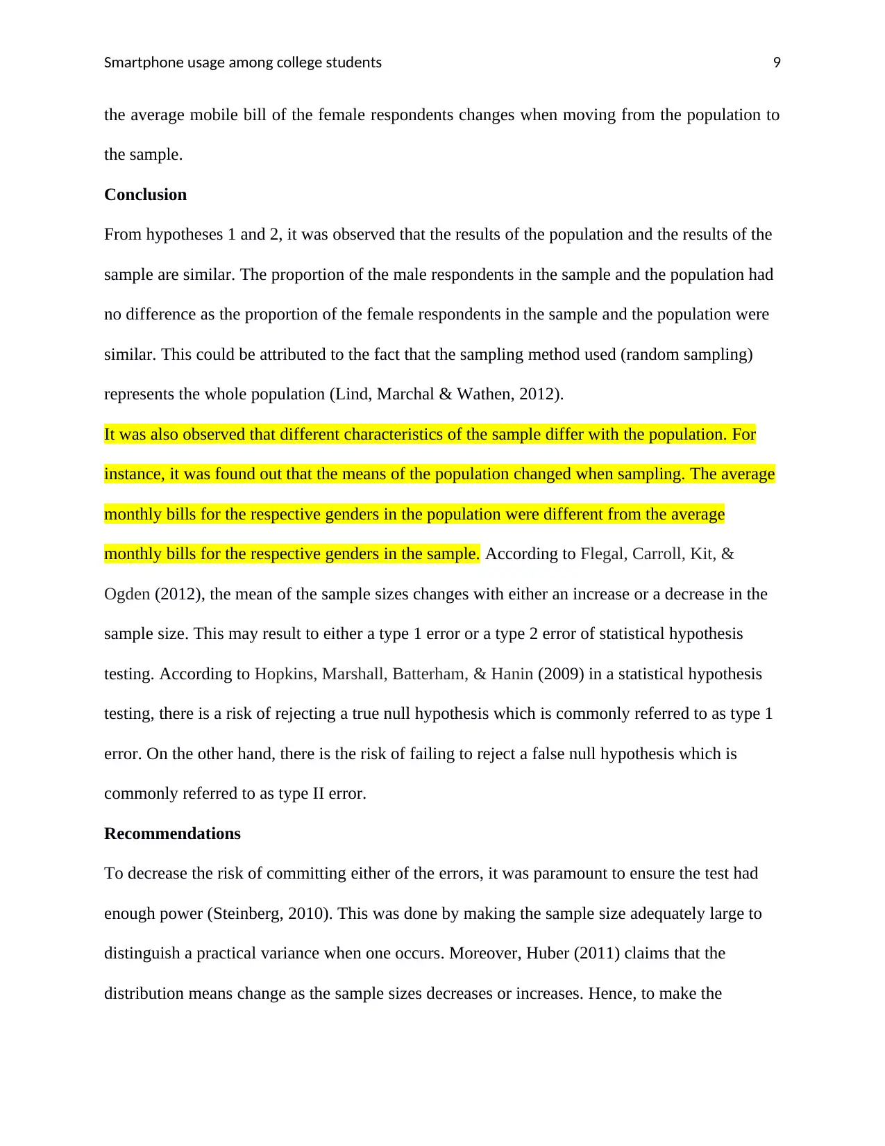
Smartphone usage among college students 9
the average mobile bill of the female respondents changes when moving from the population to
the sample.
Conclusion
From hypotheses 1 and 2, it was observed that the results of the population and the results of the
sample are similar. The proportion of the male respondents in the sample and the population had
no difference as the proportion of the female respondents in the sample and the population were
similar. This could be attributed to the fact that the sampling method used (random sampling)
represents the whole population (Lind, Marchal & Wathen, 2012).
It was also observed that different characteristics of the sample differ with the population. For
instance, it was found out that the means of the population changed when sampling. The average
monthly bills for the respective genders in the population were different from the average
monthly bills for the respective genders in the sample. According to Flegal, Carroll, Kit, &
Ogden (2012), the mean of the sample sizes changes with either an increase or a decrease in the
sample size. This may result to either a type 1 error or a type 2 error of statistical hypothesis
testing. According to Hopkins, Marshall, Batterham, & Hanin (2009) in a statistical hypothesis
testing, there is a risk of rejecting a true null hypothesis which is commonly referred to as type 1
error. On the other hand, there is the risk of failing to reject a false null hypothesis which is
commonly referred to as type II error.
Recommendations
To decrease the risk of committing either of the errors, it was paramount to ensure the test had
enough power (Steinberg, 2010). This was done by making the sample size adequately large to
distinguish a practical variance when one occurs. Moreover, Huber (2011) claims that the
distribution means change as the sample sizes decreases or increases. Hence, to make the
⊘ This is a preview!⊘
Do you want full access?
Subscribe today to unlock all pages.
Trusted by 1+ million students worldwide

Smartphone usage among college students 10
research more ssuccessful, the researcher should opt to enhance the sample size making it to be a
more representative of the whole population (Wilcox, 2010).
research more ssuccessful, the researcher should opt to enhance the sample size making it to be a
more representative of the whole population (Wilcox, 2010).
Paraphrase This Document
Need a fresh take? Get an instant paraphrase of this document with our AI Paraphraser
Smartphone usage among college students 11
References
Flegal, K. M., Carroll, M. D., Kit, B. K., & Ogden, C. L. (2012). Prevalence of obesity
and trends in the distribution of body mass index among US adults, 1999-
2010. Jama, 307(5), 491-497.
Hopkins, W., Marshall, S., Batterham, A., & Hanin, J. (2009). Progressive statistics for
studies in sports medicine and exercise science. Medicine+ Science in Sports+
Exercise, 41(1), 3.
Huber, P. J. (2011). Robust statistics. In International Encyclopedia of Statistical
Science (pp. 1248-1251). Springer, Berlin, Heidelberg.
Lind, D. A., Marchal, W. G., & Wathen, S. A. (2012). Statistical techniques in business &
economics. New York, NY: McGraw-Hill/Irwin.
Park, B. W., & Lee, K. C. (2011). The effect of users’ characteristics and experiential factors on
the compulsive usage of the smartphone. In International Conference on Ubiquitous
Computing and Multimedia Applications (pp. 438-446). Springer, Berlin, Heidelberg.
Steinberg, W. J. (2010). Student Study Guide to Accompany Statistics Alive! 2e by Wendy J.
Steinberg. Sage.
Wilcox, R. R. (2010). Fundamentals of modern statistical methods: Substantially improving
power and accuracy. Springer.
1 out of 11
Related Documents


Your All-in-One AI-Powered Toolkit for Academic Success.
+13062052269
info@desklib.com
Available 24*7 on WhatsApp / Email
![[object Object]](/_next/static/media/star-bottom.7253800d.svg)
Unlock your academic potential
Copyright © 2020–2026 A2Z Services. All Rights Reserved. Developed and managed by ZUCOL.