Statistics Homework: Probability Analysis of Student Arrival Times

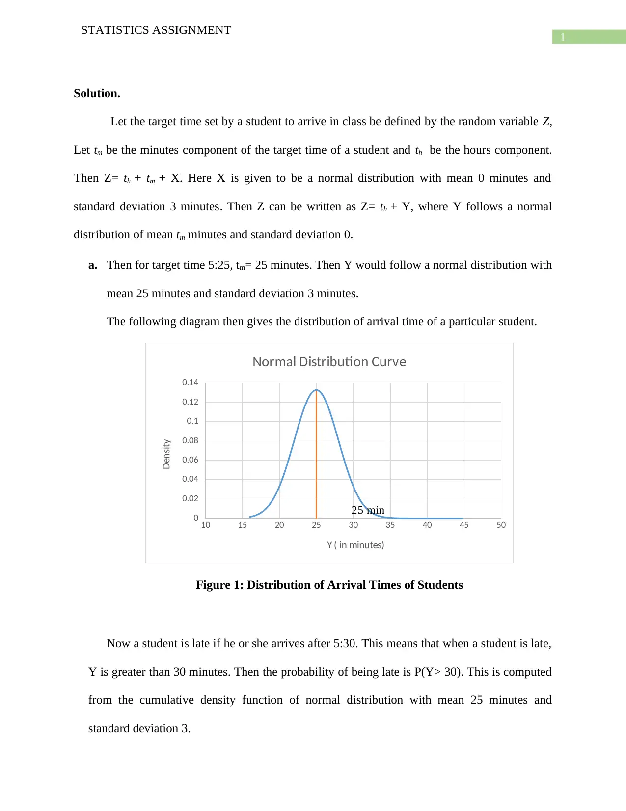
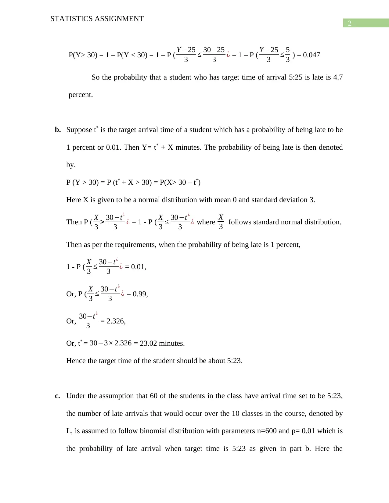
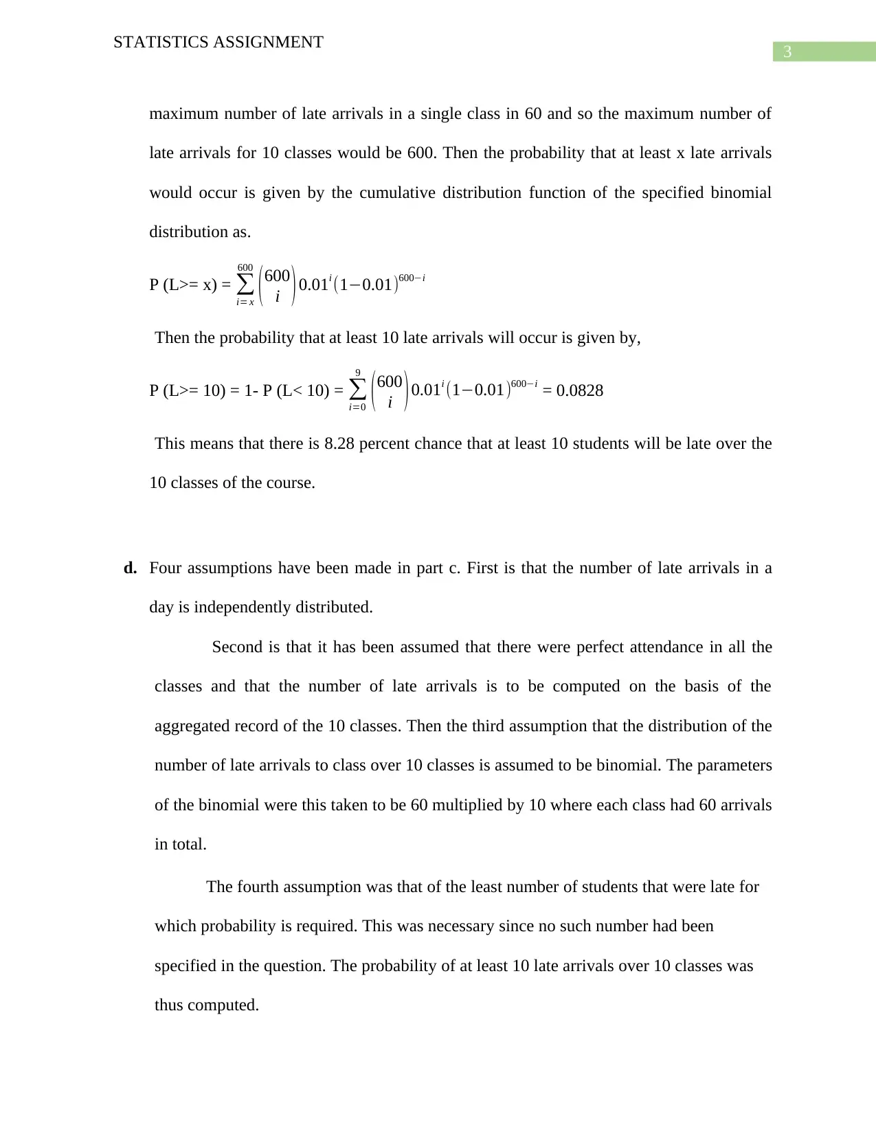
This statistics assignment delves into the analysis of student arrival times using probability distributions. It begins by modeling a student's arrival time as a normal distribution, calculating the probability of a student being late given a target arrival time. The assignment then determines the target arrival time needed to achieve a specific lateness probability. Furthermore, it explores the probability of a certain number of late arrivals occurring over multiple classes, assuming a binomial distribution. Finally, the assignment critically evaluates the assumptions made in the binomial distribution model, particularly focusing on the independence of late arrivals and highlighting the potential influence of individual behavior on attendance patterns. Desklib provides access to similar solved assignments and study resources for students.

Running head: STATISTICS ASSIGNMENT
STATISTICS ASSIGNMENT
Name of Student
Name of University
Author Note

1
STATISTICS ASSIGNMENT
Solution.
Let the target time set by a student to arrive in class be defined by the random variable Z,
Let tm be the minutes component of the target time of a student and th be the hours component.
Then Z= th + tm + X. Here X is given to be a normal distribution with mean 0 minutes and
standard deviation 3 minutes. Then Z can be written as Z= th + Y, where Y follows a normal
distribution of mean tm minutes and standard deviation 0.
a. Then for target time 5:25, tm= 25 minutes. Then Y would follow a normal distribution with
mean 25 minutes and standard deviation 3 minutes.
The following diagram then gives the distribution of arrival time of a particular student.
10 15 20 25 30 35 40 45 50
0
0.02
0.04
0.06
0.08
0.1
0.12
0.14
Normal Distribution Curve
Y ( in minutes)
Density
25 min
Figure 1: Distribution of Arrival Times of Students
Now a student is late if he or she arrives after 5:30. This means that when a student is late,
Y is greater than 30 minutes. Then the probability of being late is P(Y> 30). This is computed
from the cumulative density function of normal distribution with mean 25 minutes and
standard deviation 3.

2
STATISTICS ASSIGNMENT
P(Y> 30) = 1 – P(Y ≤ 30) = 1 – P ( Y −25
3 ≤ 30−25
3 ¿ = 1 – P ( Y −25
3 ≤ 5
3 ) = 0.047
So the probability that a student who has target time of arrival 5:25 is late is 4.7
percent.
b. Suppose t* is the target arrival time of a student which has a probability of being late to be
1 percent or 0.01. Then Y= t* + X minutes. The probability of being late is then denoted
by,
P (Y > 30) = P (t* + X > 30) = P(X> 30 – t*)
Here X is given to be a normal distribution with mean 0 and standard deviation 3.
Then P ( X
3 > 30−t¿
3 ¿ = 1 - P ( X
3 ≤ 30−t¿
3 ¿ where X
3 follows standard normal distribution.
Then as per the requirements, when the probability of being late is 1 percent,
1 - P ( X
3 ≤ 30−t¿
3 ¿ = 0.01,
Or, P ( X
3 ≤ 30−t¿
3 ¿ = 0.99,
Or, 30−t¿
3 = 2.326,
Or, t* = 30−3× 2.326 = 23.02 minutes.
Hence the target time of the student should be about 5:23.
c. Under the assumption that 60 of the students in the class have arrival time set to be 5:23,
the number of late arrivals that would occur over the 10 classes in the course, denoted by
L, is assumed to follow binomial distribution with parameters n=600 and p= 0.01 which is
the probability of late arrival when target time is 5:23 as given in part b. Here the

3
STATISTICS ASSIGNMENT
maximum number of late arrivals in a single class in 60 and so the maximum number of
late arrivals for 10 classes would be 600. Then the probability that at least x late arrivals
would occur is given by the cumulative distribution function of the specified binomial
distribution as.
P (L>= x) = ∑
i= x
600
( 600
i ) 0.01i (1−0.01)600−i
Then the probability that at least 10 late arrivals will occur is given by,
P (L>= 10) = 1- P (L< 10) = ∑
i=0
9
(600
i )0.01i (1−0.01)600−i = 0.0828
This means that there is 8.28 percent chance that at least 10 students will be late over the
10 classes of the course.
d. Four assumptions have been made in part c. First is that the number of late arrivals in a
day is independently distributed.
Second is that it has been assumed that there were perfect attendance in all the
classes and that the number of late arrivals is to be computed on the basis of the
aggregated record of the 10 classes. Then the third assumption that the distribution of the
number of late arrivals to class over 10 classes is assumed to be binomial. The parameters
of the binomial were this taken to be 60 multiplied by 10 where each class had 60 arrivals
in total.
The fourth assumption was that of the least number of students that were late for
which probability is required. This was necessary since no such number had been
specified in the question. The probability of at least 10 late arrivals over 10 classes was
thus computed.

4
STATISTICS ASSIGNMENT
The first assumption is however at risk of being true. This is because attendance is
dependent on human behavior which is inherently variable and thus attendance in itself is
variable and depends on human behavior and activity. A person may be predisposed to
being late and so timely attendance on a day would depend on their behavior in previous
classes.