Research Report: Factors Affecting Student Exam Performance Analysis

This research report presents a comprehensive statistical analysis of student exam performance, investigating gender differences and other influential factors. The study employs various statistical techniques, including t-tests and regression analysis, to examine the impact of gender, degree type...Read More

RESEARCH REPORT

Table of Contents
INTRODUCTION.........................................................................................................................................1
TASK 1 T-Test..............................................................................................................................................2
1..................................................................................................................................................................2
2 (a)............................................................................................................................................................3
2(b).............................................................................................................................................................3
2(c).............................................................................................................................................................3
2 (d). Graphical presentation and discussion.............................................................................................4
TASK 2 REGRESSION................................................................................................................................5
A. Regression output..................................................................................................................................5
B. Interpretation.........................................................................................................................................5
A. Overall adequacy of the regression model............................................................................................5
B. Interpreting regression coefficient and comment upon it presenting their statistical significance.......7
C. Comment on the changes......................................................................................................................8
TASK 3 FURTHER ANALYSIS..................................................................................................................8
CONCLUSION..............................................................................................................................................9
REFERENCES............................................................................................................................................10
APPENDIX..................................................................................................................................................11
Appendix 1: One-sample t-test................................................................................................................11
Appendix 1(2A): Independent sample t-test............................................................................................11
Appendix 1(2B): Independent sample t-test............................................................................................12
Appendix 1(2C): Independent sample t-test............................................................................................12
Appendix 2(A). Stepwise regression.......................................................................................................13
Appendix: 3..............................................................................................................................................16
1

INTRODUCTION
Data analysis is the process whereby analyst uses different techniques of statistics covering both
descriptive and inferential to examine the available dataset. It provides a strong foundation for developing
statistical literacy and statistical thinking which is essential for the business success. Research study
conducted by Buckley (2016), reported that on an average, 15-years old female students achieved
comparatively less marks than that of male candidates. However, in really, many-times, girls perform
better than boys by achieving high grades and prove the stereotype false. Therefore, the current research
report aims at investigation gender differences and also different factors that affect exam performance of
the students. For this, data have been collected about student grades, gender, degree type and lecture
attendance among different countries.
TASK 1 T-Test
1.
Step: 1: Null hypothesis
H0: The different between average marks of the student in year 2014 and 2015 is equals to zero.
(μ=29.4)
Step 2: Alternative hypothesis
H1: Average marks of the student in mathematics in 2015 are less than average student’s marks (29.4) in
2014. (μ<μ 0) (μ<29.4)
Step 3: Appropriate test: One-sample T test
Step 4: Decision rule:
This is a lower tailed test at 5% level of significance. If p-value is below 0.05 then null
hypothesis will be rejected, otherwise, accepted.
Step: 5. Computation of test statistics
Appendix 1.
Step: 6. Conclusion
As per the results, in 2015, average marks of the students is 28.76 (S . D.=12.335) which is less
than average students marks of 29.4 in 2014. Looking to the one-sample test results, P=0.171>0.05, it
2

is therefore, decision rule accepted null hypothesis stating that there is no significant level of mean
differences exists in the average marks of the students in 2014 and 2015 (Keller, 2014).
2 (a)
H0: There is no significant mean difference exists between marks obtained by female and male students.
(μ1=μ 2)
H0: There is significant mean difference exists between marks obtained by female and male students.
(μ1=μ 2)
Statistical Test: Two Sample t-test / Independent sample t-test
Test statistics:  = 5%.
Results
Appendix 1.(2A)
There are 340 male and 354 female students who achieved mean score of 27.76 and 29.72 with a
standard deviation of 12.398 and 12.215 respectively. Under the leneve’s test, sig. value is 0.926 at
(P=0.036<0.05) that implies that there is difference in the average marks achieved by female and male
significantly differ from each other, hence, null hypothesis rejected and alternative accepted.
2(b)
H0: There is no significant difference in the average marks of male and female belonged to single degree
students.
H1: There is significant difference in the average marks of male and female belonged to single degree
students.
Statistical Test: Two Sample t-test / Independent sample t-test
Test statistics:  = 5%.
Results:
Appendix 1(2B)
Interpretation: There is 242 and 216 single degree holder male and female whose average marks
in mathematics is 27.10 and 27.12 at S.D. of 12.565 and 11.330. Both categories showed close value of
mean and discovered P value to 0.982>0.05, therefore, it can be said that there are enough evidence
available to accept null hypothesis (Aczel and Sounderpandian, 2002 ). Thus, there is no different
between average exam performances between female and male of single degree students.
3

2(c)
H0: There is no significant difference in the average marks of male and female belonged to double degree
students.
H1: There is significant difference in the average marks of male and female belonged to double degree
students.
Statistical Test: Two Sample t-test / Independent sample t-test
Test statistics:  = 5%.
Results:
Appendix 1(2C)
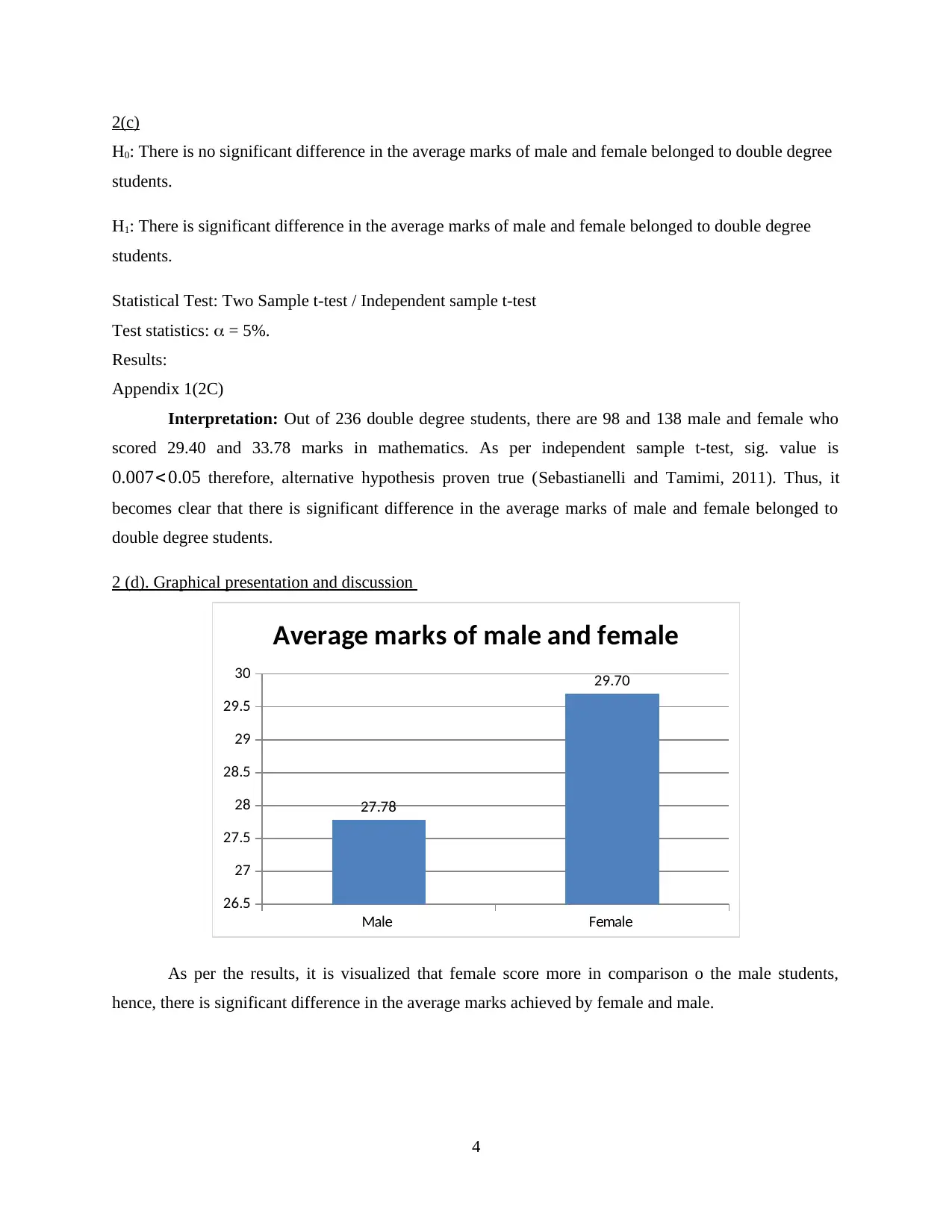
Interpretation: Out of 236 double degree students, there are 98 and 138 male and female who
scored 29.40 and 33.78 marks in mathematics. As per independent sample t-test, sig. value is
0.007< 0.05 therefore, alternative hypothesis proven true (Sebastianelli and Tamimi, 2011). Thus, it
becomes clear that there is significant difference in the average marks of male and female belonged to
double degree students.
2 (d). Graphical presentation and discussion
Male Female
26.5
27
27.5
28
28.5
29
29.5
30
27.78
29.70
Average marks of male and female
As per the results, it is visualized that female score more in comparison o the male students,
hence, there is significant difference in the average marks achieved by female and male.
4

Male Female Male Female
Single Double
0
5
10
15
20
25
30
35
40
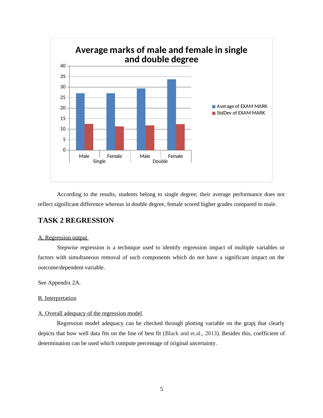
Average marks of male and female in single
and double degree
Average of EXAM MARK
StdDev of EXAM MARK
According to the results, students belong to single degree; their average performance does not
reflect significant difference whereas in double degree, female scored higher grades compared to male.
TASK 2 REGRESSION
A. Regression output
Stepwise regression is a technique used to identify regression impact of multiple variables or
factors with simultaneous removal of such components which do not have a significant impact on the
outcome/dependent variable.
See Appendix 2A.
B. Interpretation
A. Overall adequacy of the regression model
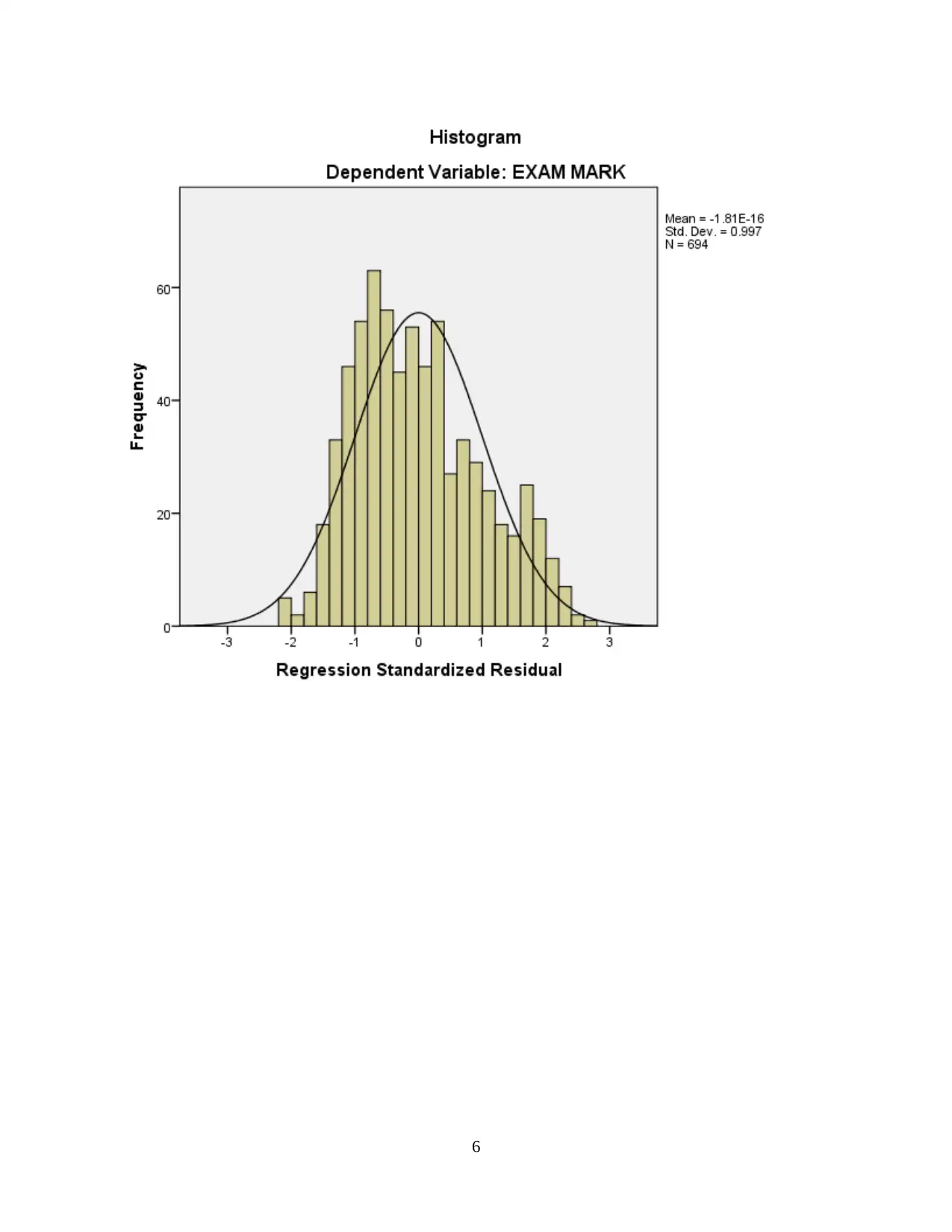
Regression model adequacy can be checked through plotting variable on the grapj that clearly
depicts that how well data fits on the line of best fit (Black and et.al., 2013). Besides this, coefficient of
determination can be used which compute percentage of original uncertainty.
5

6

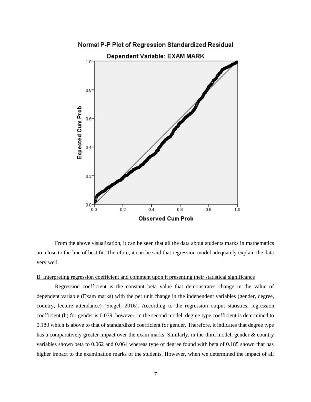
From the above visualization, it can be seen that all the data about students marks in mathematics
are close to the line of best fit. Therefore, it can be said that regression model adequately explain the data
very well.
B. Interpreting regression coefficient and comment upon it presenting their statistical significance
Regression coefficient is the constant beta value that demonstrates change in the value of
dependent variable (Exam marks) with the per unit change in the independent variables (gender, degree,
country, lecture attendance) (Siegel, 2016). According to the regression output statistics, regression
coefficient (b) for gender is 0.079, however, in the second model, degree type coefficient is determined to
0.180 which is above to that of standardized coefficient for gender. Therefore, it indicates that degree type
has a comparatively greater impact over the exam marks. Similarly, in the third model, gender & country
variables shown beta to 0.062 and 0.064 whereas type of degree found with beta of 0.185 shown that has
higher impact to the examination marks of the students. However, when we determined the impact of all
7

the four variables on the marks, then beta value for lecture attendance and degree type is reported to 0.176
and 0.168 which is higher to degree with coefficient of 0.051 and country of citizenship with 0.059. Thus,
it shows that out of all the variables, lecture attendance and degree type highly influence student’s grades
(Keller, 2016).
C. Comment on the changes
As per the results, initially, gender shown regression coefficient of 0.079 at a sig value of
0.036<0.05 which indicates gender affects examination performance. It also can be evident from the t-test
results which found P value of 0.036 and accept alternative hypothesis accepting that average student’s
marks of female and male vary from each other. However, when degree type is included, it’s coefficient
has been decreased to 0.060 and degree type shown coefficient of 0.180 at a sig value of 0.000 reflecting
that there is significant difference in the candidate’s performance belonging to different degree type. In
the third model, country is also included, as a result, coefficient for both gender and degree type goes up
to 0.162 and 0.185 at zero level of sig accept alternative hypothesis (Lai, Zhu and Williams, 2017).
Lastly, gender, type of degree, country and lecture attendance were being tested, provided P value to 0.00
hence, it becomes clear that all the factors significantly affect exam performance of the students.
TASK 3 FURTHER ANALYSIS
As per the above regression model, significant impact has been founded at a P=0.000 covering all
the variables. However, evidencing it from the earlier findings in t-test, no different is found for the single
degree student’s male and female performance whereas double degree students found significant
difference in the results. Therefore, it results in a suspicion that gender, country of citizenship and lecture
attendance’s effect on exam performance may be dependent on or interact with degree type. Therefore, in
order to find out their impact, regression test needs to be performed separately as follows:
In order to find regression separately in SPSS for the nominal variables, a number of k −1dummy
variables needs to be put. Here, degree type is a nominal variable and there are two Ks, single and double
degree, therefore, 2-1 = 1 dummy variable needs to be created. The dummy variable is provided as
follows:
Degree type Original Dummy
Single 1 2
Double 2 1
8

Initially, regression is performed to examine the impact of degree type on the student’s marks
(shown∈ Appendix 3). The regression results determined unstandardized coefficient of 4.855. For both
the degree type, regression equation is performed as below:
= b0 + b1 (Degree type)
Single degree type = 22.252 + 4.855(1)
= 27.107
Double degree type = 22.252 + 4.855(2)
= 31.962
Performing independent sample t-test, mean difference at t value of -4.996 under equal variance
is found to -4.855 which is exactly same to that of coefficient in simple linear regression except only the
reversed signs. Similarly, univariate analysis is performed which found f value of 24.960 for the degree
type exactly same to the square of t-value (−4.996 2) and Parameter estimates determined beta value to -
4.855. It clearly showcase that F statistics under Univariate ANOVA results shows the same results under
t-test. It found intercept of 31.962 which matches regression for double degree type (see above).
Afterwards, the variable degree type is recoded in which only double degree type is minimized from 2 to
0. After performing univariate ANOVA again, regression value is equal to earlier to 4.855 at an intercept
of 27.107 for the single degree type. It clearly presents that regression equation always use intercepts for
the higher value.
CONCLUSION
Results determined no significant level of mean differences exists in the average marks of the
students in 2014 and 2015. However, significant difference is found between average marks achieved by
female and male students. Multiple regressions determined that independent variables like gender, degree
type, citizenship and lecture attendance have a significant impact student’s exam performance.
9

REFERENCES
Books and Journals
Aczel, A. D. and Sounderpandian, 2002. Complete business statistics. McGraw-Hill/Irwin.
Black, K and et.al., 2013. Australasian business statistics. John Wiley & Sons.
Keller, G., 2014. Statistics for management and economics. Nelson Education.
Keller, G., 2016. Modern Business Statistics. McGraw-Hill/Irwin.
Lai, G., Zhu, Z. and Williams, D. 2017. Enhance Students’ Learning in Business Statistics Class Using
Video Tutorials. Journal of Teaching and Learning with Technology. 6(1). 31-44.
Sebastianelli, R. and Tamimi, N., 2011. Business statistics and management science online: Teaching
strategies and assessment of student learning. Journal of Education for Business. 86(6). pp.317-
325.
Siegel, A., 2016. Practical business statistics. Academic Press.
10

APPENDIX
Appendix 1: One-sample t-test
One-Sample Statistics
N Mean Std. Deviation Std. Error Mean
EXAM MARK 694 28.76 12.335 .468
One-Sample Test
Test Value = 29.4
t df Sig. (2-
tailed)
Mean Difference 95% Confidence Interval of the
Difference
Lower Upper
EXAM
MARK -1.371 693 .171 -.642 -1.56 .28
Appendix 1(2A): Independent sample t-test
Group Statistics
Gender N Mean Std. Deviation Std. Error Mean
EXAM MARK Male 340 27.76 12.398 .672
Female 354 29.72 12.215 .649
Independent Samples Test
Levene's Test
for Equality of
Variances
t-test for Equality of Means
F Sig. t df Sig.
(2-
tailed)
Mean
Differenc
e
Std. Error
Differenc
e
95%
Confidence
Interval of the
Difference
Lower Upper
EXAM
MAR
K
Equal
variances
assumed
.009 .926 -
2.09
6
692 .036 -1.959 .934 -3.793 -.124
11

Equal
variances not
assumed
-
2.09
6
689.89
3 .036 -1.959 .935 -3.794 -.124
Appendix 1(2B): Independent sample t-test
Group Statisticsa
Gender N Mean Std. Deviation Std. Error Mean
EXAM MARK Male 242 27.10 12.565 .808
Female 216 27.12 11.330 .771
a. Degree Type = Single
Independent Samples Testa
Levene's
Test for
Equality of
Variances
t-test for Equality of Means
F Sig. t df Sig.
(2-
tailed)
Mean
Difference
Std. Error
Difference
95%
Confidence
Interval of the
Difference
Lower Upper
EXAM
MARK
Equal
variances
assumed
3.653 .057 -.02
3 456 .982 -.025 1.123 -2.232 2.182
Equal
variances
not
assumed
-.02
3 455.950 .982 -.025 1.117 -2.220 2.169
a. Degree Type = Single
Appendix 1(2C): Independent sample t-test
12

Group Statisticsa
Gender N Mean Std. Deviation Std. Error Mean
EXAM MARK Male 98 29.40 11.880 1.200
Female 138 33.78 12.479 1.062
a. Degree Type = Double
Independent Samples Testa
Levene's Test
for Equality of
Variances
t-test for Equality of Means
F Sig. t df Sig.
(2-
tailed)
Mean
Differenc
e
Std. Error
Differenc
e
95%
Confidence
Interval of the
Difference
Lower Upper
EXAM
MAR
K
Equal
variances
assumed
1.208 .273
-
2.71
3
234 .007 -4.385 1.616 -7.569 -1.201
Equal
variances not
assumed
-
2.73
6
215.07
2 .007 -4.385 1.603 -7.544 -1.226
a. Degree Type = Double
Appendix 2(A). Stepwise regression
Model Summarye
Model R R Square Adjusted R Square Std. Error of the
Estimate
1 .079a .006 .005 12.305
2 .196b .038 .036 12.114
3 .206c .042 .038 12.097
4 .270d .073 .068 11.911
a. Predictors: (Constant), Gender
13

b. Predictors: (Constant), Gender, Degree Type
c. Predictors: (Constant), Gender, Degree Type, Country
d. Predictors: (Constant), Gender, Degree Type, Country, Lecture Attendance
e. Dependent Variable: EXAM MARK
ANOVAa
Model Sum of Squares df Mean Square F Sig.
1
Regression 665.356 1 665.356 4.394 .036b
Residual 104779.975 692 151.416
Total 105445.331 693
2
Regression 4047.699 2 2023.849 13.792 .000c
Residual 101397.632 691 146.740
Total 105445.331 693
3
Regression 4471.235 3 1490.412 10.185 .000d
Residual 100974.096 690 146.339
Total 105445.331 693
4
Regression 7703.093 4 1925.773 13.575 .000e
Residual 97742.238 689 141.861
Total 105445.331 693
a. Dependent Variable: EXAM MARK
b. Predictors: (Constant), Gender
c. Predictors: (Constant), Gender, Degree Type
d. Predictors: (Constant), Gender, Degree Type, Country
e. Predictors: (Constant), Gender, Degree Type, Country, Lecture Attendance
Coefficientsa
Model Unstandardized
Coefficients
Standardize
d
Coefficients
t Sig. Collinearity
Statistics
B Std. Error Beta Toleranc
e
VIF
1 (Constant) 25.800 1.486 17.359 .000
14

Gender 1.959 .934 .079 2.096 .036 1.000 1.000
2
(Constant) 20.238 1.866 10.844 .000
Gender 1.482 .925 .060 1.602 .110 .989 1.012
Degree Type 4.687 .976 .180 4.801 .000 .989 1.012
3
(Constant) 18.206 2.214 8.225 .000
Gender 1.533 .924 .062 1.659 .098 .987 1.013
Degree Type 4.815 .978 .185 4.924 .000 .983 1.018
Country 1.394 .819 .064 1.701 .089 .992 1.008
4
(Constant) 13.976 2.353 5.940 .000
Gender 1.252 .912 .051 1.373 .170 .983 1.017
Degree Type 4.382 .967 .168 4.532 .000 .974 1.027
Country 1.285 .807 .059 1.593 .112 .992 1.008
Lecture
Attendance .767 .161 .176 4.773 .000 .985 1.015
a. Dependent Variable: EXAM MARK
Excluded Variablesa
Model Beta In t Sig. Partial
Correlation
Collinearity Statistics
Tolerance VIF Minimum
Tolerance
1
Degree Type .180b 4.801 .000 .180 .989 1.012 .989
Country .049b 1.304 .193 .050 .998 1.002 .998
Lecture
Attendance .193b 5.173 .000 .193 .995 1.005 .995
2
Country .064c 1.701 .089 .065 .992 1.008 .983
Lecture
Attendance .178c 4.814 .000 .180 .986 1.014 .980
3 Lecture
Attendance .176d 4.773 .000 .179 .985 1.015 .974
a. Dependent Variable: EXAM MARK
b. Predictors in the Model: (Constant), Gender
c. Predictors in the Model: (Constant), Gender, Degree Type
15

d. Predictors in the Model: (Constant), Gender, Degree Type, Country
Collinearity Diagnosticsa
Mode
l
Dimensio
n
Eigenvalu
e
Condition
Index
Variance Proportions
(Constant
)
Gender Degree
Type
Country Lecture
Attendance
1 1 1.949 1.000 .03 .03
2 .051 6.203 .97 .97
2
1 2.866 1.000 .01 .01 .01
2 .094 5.522 .00 .47 .63
3 .040 8.436 .99 .51 .36
3
1 3.716 1.000 .00 .01 .01 .01
2 .159 4.831 .00 .06 .14 .71
3 .093 6.318 .00 .56 .54 .02
4 .032 10.832 1.00 .38 .32 .27
4
1 4.595 1.000 .00 .00 .00 .01 .01
2 .164 5.299 .00 .03 .08 .75 .07
3 .120 6.199 .00 .10 .15 .00 .81
4 .093 7.026 .00 .57 .52 .01 .00
5 .029 12.613 1.00 .30 .24 .23 .12
a. Dependent Variable: EXAM MARK
Residuals Statisticsa
Minimum Maximum Mean Std. Deviation N
Predicted Value 20.90 36.77 28.76 3.334 694
Residual -25.180 31.202 .000 11.876 694
Std. Predicted Value -2.358 2.403 .000 1.000 694
Std. Residual -2.114 2.620 .000 .997 694
a. Dependent Variable: EXAM MARK
Appendix: 3
16

Variables Entered/Removeda
Model Variables Entered Variables Removed Method
1 Degree Typeb . Enter
a. Dependent Variable: EXAM MARK
b. All requested variables entered.
Model Summary
Model R R Square Adjusted R Square Std. Error of the Estimate
1 .187a .035 .033 12.127
a. Predictors: (Constant), Degree Type
ANOVAa
Model Sum of Squares df Mean Square F Sig.
1
Regression 3670.917 1 3670.917 24.960 .000b
Residual 101774.414 692 147.073
Total 105445.331 693
a. Dependent Variable: EXAM MARK
b. Predictors: (Constant), Degree Type
Coefficientsa
Model Unstandardized Coefficients Standardized
Coefficients
t Sig.
B Std. Error Beta
1 (Constant) 22.252 1.381 16.111 .000
Degree Type 4.855 .972 .187 4.996 .000
a. Dependent Variable: EXAM MARK
Univariate analysis of variance
Between-Subjects Factors
17

Value Label N
Degree Type 1 Single 458
2 Double 236
Tests of Between-Subjects Effects
Dependent Variable: EXAM MARK
Source Type III Sum of
Squares
df Mean Square F Sig.
Corrected Model 3670.917a 1 3670.917 24.960 .000
Intercept 543419.303 1 543419.303 3694.899 .000
DegreeType 3670.917 1 3670.917 24.960 .000
Error 101774.414 692 147.073
Total 679396.000 694
Corrected Total 105445.331 693
a. R Squared = .035 (Adjusted R Squared = .033)
Parameter Estimates
Dependent Variable: EXAM MARK
Parameter B Std. Error t Sig. 95% Confidence Interval
Lower Bound Upper Bound
Intercept 31.962 .789 40.488 .000 30.412 33.512
[DegreeType=1] -4.855 .972 -4.996 .000 -6.763 -2.947
[DegreeType=2] 0a . . . . .
a. This parameter is set to zero because it is redundant.
Independent sample t-test
Group Statistics
Degree Type N Mean Std. Deviation Std. Error Mean
EXAM
MARK
Single 458 27.11 11.986 .560
Double 236 31.96 12.398 .807
18

Independent Samples Test
Levene's
Test for
Equality of
Variances
t-test for Equality of Means
F Sig. t df Sig.
(2-
tailed)
Mean
Differenc
e
Std. Error
Differenc
e
95%
Confidence
Interval of
the
Difference
Lowe
r
Upper
EXAM
MARK
Equal
variances
assumed
.907 .341
-
4.99
6
692 .000 -4.855 .972 -6.763 -
2.947
Equal
variances
not
assumed
-
4.94
2
460.861 .000 -4.855 .982 -6.785 -
2.924
Univariate analysis of variances for recoded variable
Between-Subjects Factors
N
Degree type recoded .00 236
1.00 458
Tests of Between-Subjects Effects
Dependent Variable: EXAM MARK
Source Type III Sum of
Squares
df Mean Square F Sig.
Corrected Model 3670.917a 1 3670.917 24.960 .000
19