Student Weekly Rent Analysis Report: Property and Rent Insights

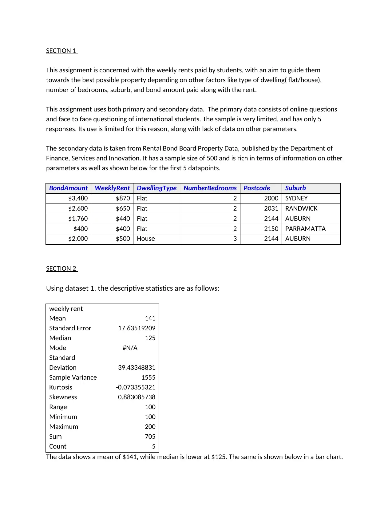
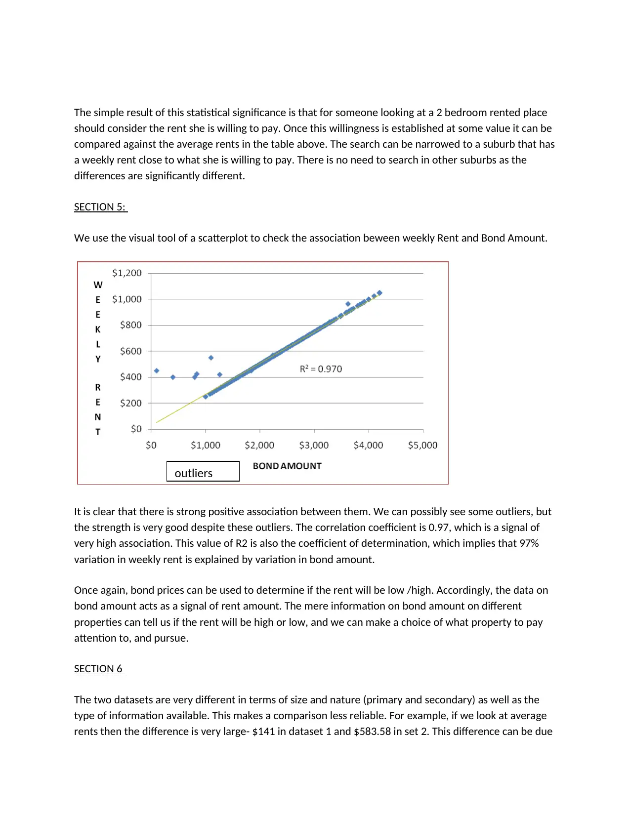
This report analyzes student weekly rents, dwelling types, and bond amounts using primary and secondary data. The primary data, though limited, provides initial insights, while the secondary data from Rental Bond Board Property Data offers a comprehensive view with a larger sample size. Descriptive statistics reveal a mean weekly rent of $141 with a positive skew. The analysis explores dwelling type preferences, highlighting the dominance of flats among students and uses a one-tail hypothesis test to show that the proportion of houses is significantly less than 0.1. Further, the report examines average weekly rents for two-bedroom properties across different suburbs using ANOVA, demonstrating statistically significant differences. Finally, the report uses a scatterplot to visualize the strong positive correlation between weekly rent and bond amount, indicating that bond amounts can be used to estimate rent. The report concludes by acknowledging the limitations of comparing the two datasets and offers recommendations for improving the primary dataset, such as increasing sample size and collecting comparable parameters.

Student name:
Course:

SECTION 1
This assignment is concerned with the weekly rents paid by students, with an aim to guide them
towards the best possible property depending on other factors like type of dwelling( flat/house),
number of bedrooms, suburb, and bond amount paid along with the rent.
This assignment uses both primary and secondary data. The primary data consists of online questions
and face to face questioning of international students. The sample is very limited, and has only 5
responses. Its use is limited for this reason, along with lack of data on other parameters.
The secondary data is taken from Rental Bond Board Property Data, published by the Department of
Finance, Services and Innovation. It has a sample size of 500 and is rich in terms of information on other
parameters as well as shown below for the first 5 datapoints.
BondAmount WeeklyRent DwellingType NumberBedrooms Postcode Suburb
$3,480 $870 Flat 2 2000 SYDNEY
$2,600 $650 Flat 2 2031 RANDWICK
$1,760 $440 Flat 2 2144 AUBURN
$400 $400 Flat 2 2150 PARRAMATTA
$2,000 $500 House 3 2144 AUBURN
SECTION 2
Using dataset 1, the descriptive statistics are as follows:
weekly rent
Mean 141
Standard Error 17.63519209
Median 125
Mode #N/A
Standard
Deviation 39.43348831
Sample Variance 1555
Kurtosis -0.073355321
Skewness 0.883085738
Range 100
Minimum 100
Maximum 200
Sum 705
Count 5
The data shows a mean of $141, while median is lower at $125. The same is shown below in a bar chart.

The highest rent is for student 3 at $200 and the lowest is $100 (just halve of the highest . The range is
thus 200-100 =100. This is relatively high. The data is a little skewed in the positive direction as shown by
a value of 0.88. for more detailed analysis and inferences we need a larger sample.
SECTION 3:
a. We first consider the data on Dwelling Type only. The table below shows a 2*2 classification across
suburbs and type of dwellings. The dominance of flats- 473/500 is clear. Almost 94.6% students live in
flats. Within suburbs, Parramatta dominates the sample. (164/500). Sydney stands out as there are no
students living in a house here.
Row Labels Flat House Grand Total
AUBURN 47 14 61
PARRAMATTA 156 8 164
RANDWICK 123 5 128
SYDNEY 147 147
Grand Total 473 27 500
The above information is also seen below in the bar chart.

The proportion of House as a dwelling type is 27/500 = 0.054
So the required sample proportion = p = 0.054
Ho: p= 0.1
H1: p < 0.1
This is a one tail (left tail) hypothesis test using the z test.
Test value = (0.054 – 0.1)/ SE where SE = (0.054 *.946 /500)^.5 = 0.0101
Test value = - 0.046/0.0101 = -4.551. The p value of this value is zero, and 0.05 > 0 which implies that at
a 5% level of significance, we do not accept the null hypothesis. There is evidence that proportion of
Houses is less than 0.1.
This test shows that the student prefer flats by an overwhelming majority- more than 90%. While we
cannot investigate the reasons here , the results are enough to recommend a flat for a new student
looking for accommodation.
SECTION 4:
b. Next we focus only on properties (flats and houses) with 2 bedrooms only. The table below show the
average weekly rents across suburbs. Auburn is the cheapest with lowest average rent of $410.68, while
Sydney is most expensive at $855.07. the bar chart shows the same information graphically in a relative
and visual sense.

AUBURN PARRAMATTA RANDWICK SYDNEY
Average of
WeeklyRent 410.68 481.76 619.94 855.07
We use ANOVA to see if the differences are statistically significant. The ANOVA results show that the F
test value is 261.97. this is much higher than the critical F value of 2.63. This leads us to conclude that
the differences in average weekly rents across the 4 suburbs are statistically different.
Anova: Single Factor
SUMMARY
Groups Count Sum Average Variance
Column 1 30 11795 393.1666667 2290.488506
Column 2 113 53580 474.159292 4371.831542
Column 3 79 48054 608.278481 11073.22915
Column 4 61 51285 840.7377049 14925.69672
ANOVA
Source of
Variation SS df MS F P-value F crit
Between Groups 6522099 3 2174032.933 261.9743312 8.1542E-81 2.63696
Within Groups 2315323 279 8298.64866
Total 8837422 282

The simple result of this statistical significance is that for someone looking at a 2 bedroom rented place
should consider the rent she is willing to pay. Once this willingness is established at some value it can be
compared against the average rents in the table above. The search can be narrowed to a suburb that has
a weekly rent close to what she is willing to pay. There is no need to search in other suburbs as the
differences are significantly different.
SECTION 5:
We use the visual tool of a scatterplot to check the association beween weekly Rent and Bond Amount.
It is clear that there is strong positive association between them. We can possibly see some outliers, but
the strength is very good despite these outliers. The correlation coefficient is 0.97, which is a signal of
very high association. This value of R2 is also the coefficient of determination, which implies that 97%
variation in weekly rent is explained by variation in bond amount.
Once again, bond prices can be used to determine if the rent will be low /high. Accordingly, the data on
bond amount acts as a signal of rent amount. The mere information on bond amount on different
properties can tell us if the rent will be high or low, and we can make a choice of what property to pay
attention to, and pursue.
SECTION 6
The two datasets are very different in terms of size and nature (primary and secondary) as well as the
type of information available. This makes a comparison less reliable. For example, if we look at average
rents then the difference is very large- $141 in dataset 1 and $583.58 in set 2. This difference can be due
outliers

to many reasons, which can beyond analysis here. As the parameters of the data points are also
different we must not use dataset 1 for any kind of inferences.
 Dataset 2 is much richer and is a good indicator and guide when looking for a property to rent.
 Dataset 1 needs to be improved along many lines:
 Sample size must be increased, and comparable with other set.
 Information must be collected on parameters that dataset 2 covers to allow comparison.
 Another piece of information that can help is the sex of the student, and the preference for
sharing the accommodation.

References
Anon., n.d. Hypothess testing. [Online] Available at: http://www.statisticshowto.com/probability-and-
statistics/hypothesis-testing/ [Accessed 12 Sep 2017].
Anon., n.d. Mean, median, mode. [Online] Available at:
http://www.bbc.co.uk/schools/gcsebitesize/maths/statistics/measuresofaveragerev6.shtml [Accessed
13 Sep 2017].
Home.iitk.ac.in, n.d. Regression analysis. [Online] Available at:
http://home.iitk.ac.in/~shalab/regression/Chapter2-Regression-SimpleLinearRegressionAnalysis.pdf
[Accessed 6 Sep 2017].
Learn,bu.edu, n.d. The 5 steps in Hypothesis testing. [Online] Available at:
https://learn.bu.edu/bbcswebdav/pid-826908-dt-content-rid-2073693_1/courses/13sprgmetcj702_ol/
week04/metcj702_W04S01T05_fivesteps.html [Accessed 5 Sep 2017].
Rgs.org, n.d. Sampling techniques. [Online] Available
athttp://www.rgs.org/OurWork/Schools/Fieldwork+and+local+learning/Fieldwork+techniques/
Sampling+techniques.htm [Accessed 15 Sep 2017].
stat.ualberta.ca, n.d. What isa P value. [Online] Available at:
http://www.stat.ualberta.ca/~hooper/teaching/misc/Pvalue.pdf [Accessed 9 Sep 2017].