MBA 5652: Data Analysis of Sun Coast Data using Parametric Tools

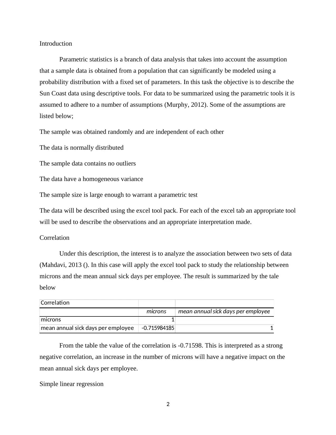
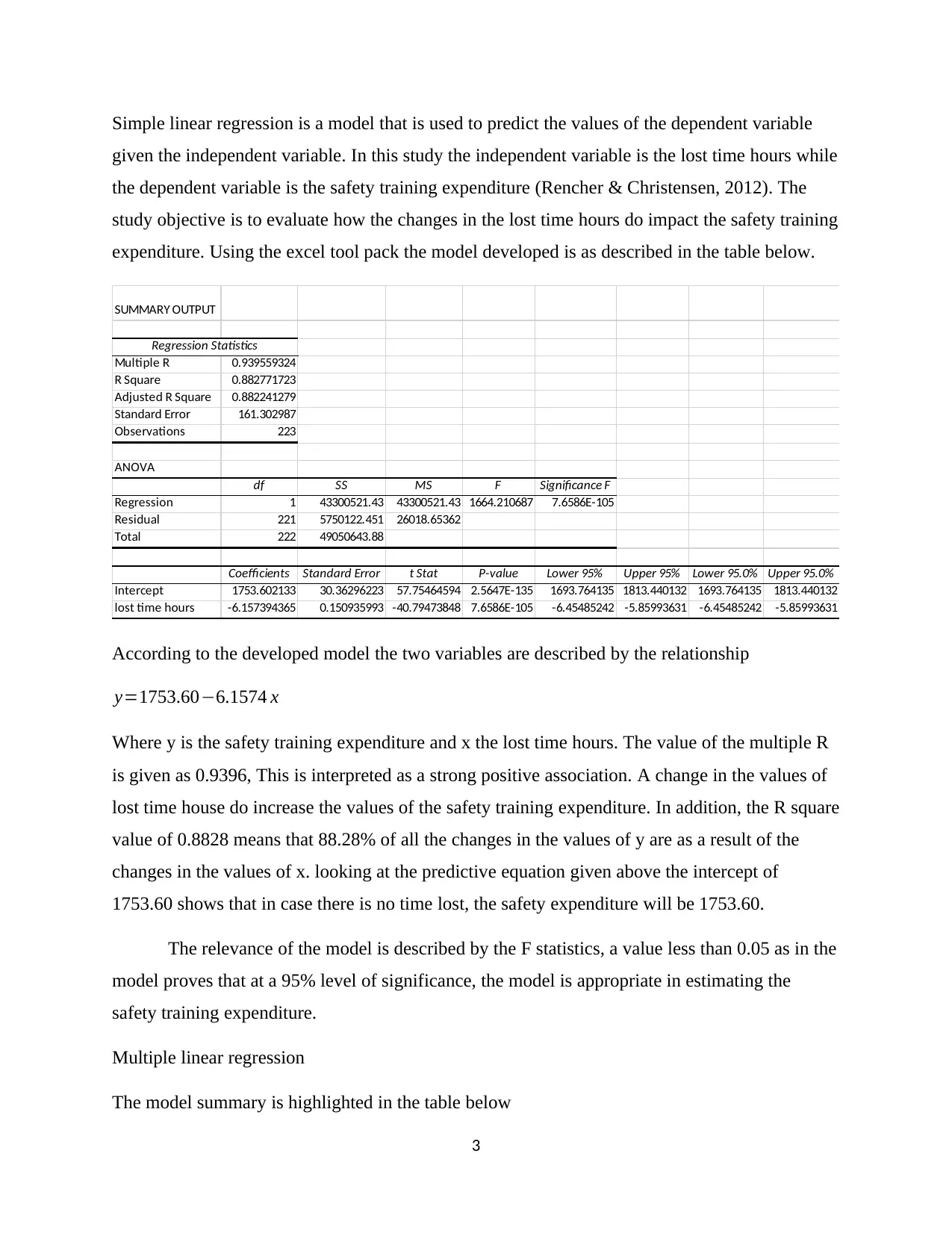
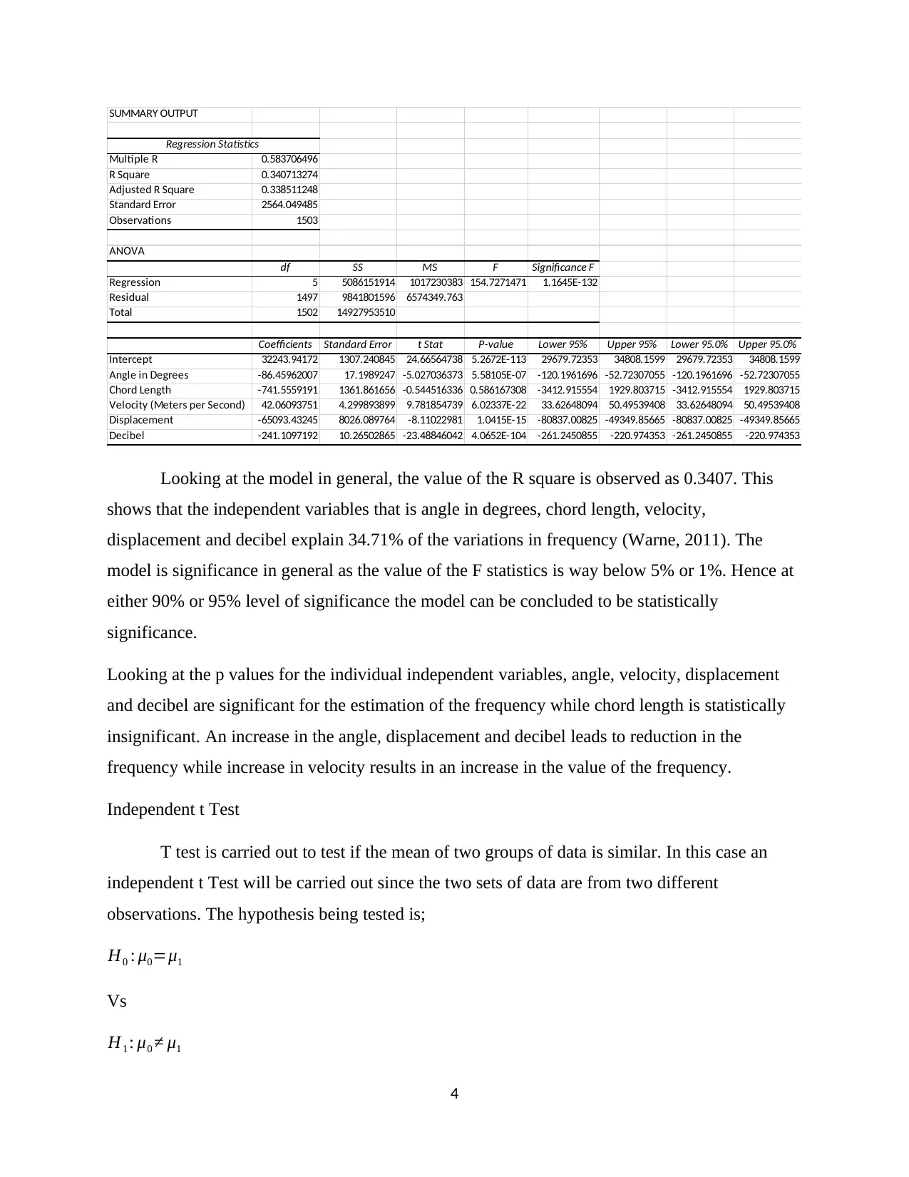
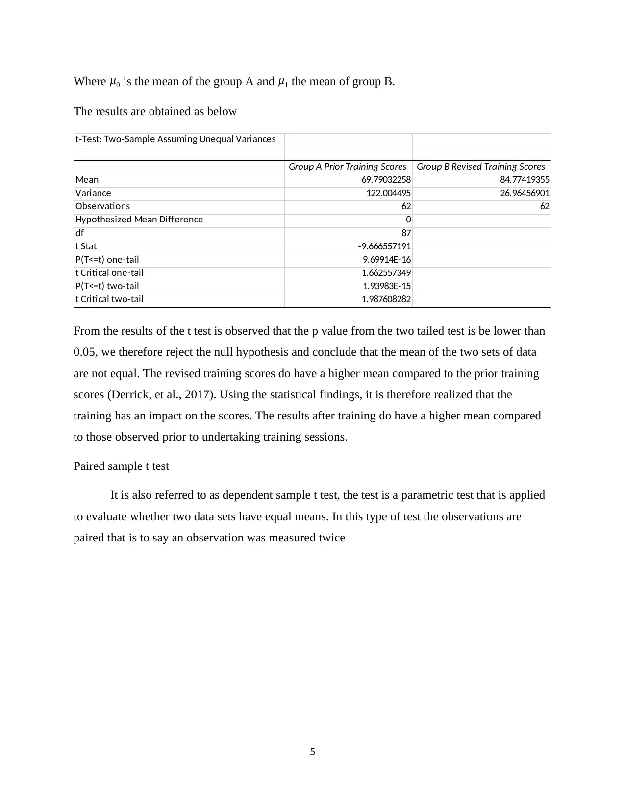
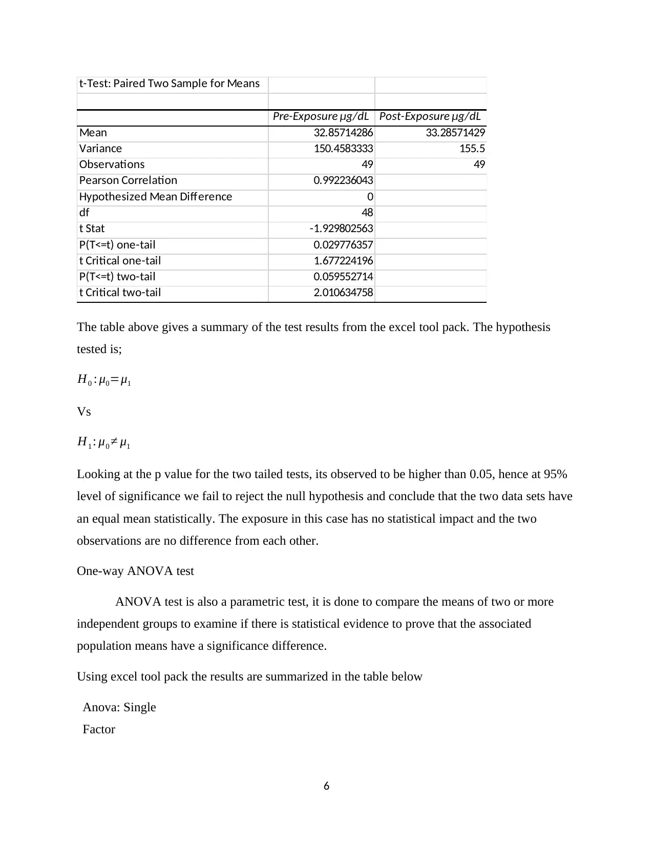
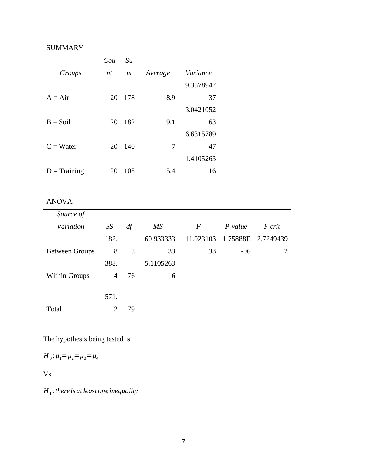
This project analyzes the Sun Coast data using parametric statistical tools within Excel. It begins with an introduction to parametric statistics, outlining the assumptions required for its application. The analysis covers correlation, examining the relationship between microns and mean annual sick da...Read More

MBA 5652-unit IV scholarly activity
Student Name
Institution Name
1

Introduction
Parametric statistics is a branch of data analysis that takes into account the assumption
that a sample data is obtained from a population that can significantly be modeled using a
probability distribution with a fixed set of parameters. In this task the objective is to describe the
Sun Coast data using descriptive tools. For data to be summarized using the parametric tools it is
assumed to adhere to a number of assumptions (Murphy, 2012). Some of the assumptions are
listed below;
The sample was obtained randomly and are independent of each other
The data is normally distributed
The sample data contains no outliers
The data have a homogeneous variance
The sample size is large enough to warrant a parametric test
The data will be described using the excel tool pack. For each of the excel tab an appropriate tool
will be used to describe the observations and an appropriate interpretation made.
Correlation
Under this description, the interest is to analyze the association between two sets of data
(Mahdavi, 2013 (). In this case will apply the excel tool pack to study the relationship between
microns and the mean annual sick days per employee. The result is summarized by the tale
below
Correlation
microns mean annual sick days per employee
microns 1
mean annual sick days per employee -0.715984185 1
From the table the value of the correlation is -0.71598. This is interpreted as a strong
negative correlation, an increase in the number of microns will have a negative impact on the
mean annual sick days per employee.
Simple linear regression
2

Simple linear regression is a model that is used to predict the values of the dependent variable
given the independent variable. In this study the independent variable is the lost time hours while
the dependent variable is the safety training expenditure (Rencher & Christensen, 2012). The
study objective is to evaluate how the changes in the lost time hours do impact the safety training
expenditure. Using the excel tool pack the model developed is as described in the table below.
SUMMARY OUTPUT
Regression Statistics
Multiple R 0.939559324
R Square 0.882771723
Adjusted R Square 0.882241279
Standard Error 161.302987
Observations 223
ANOVA
df SS MS F Significance F
Regression 1 43300521.43 43300521.43 1664.210687 7.6586E-105
Residual 221 5750122.451 26018.65362
Total 222 49050643.88
Coefficients Standard Error t Stat P-value Lower 95% Upper 95% Lower 95.0% Upper 95.0%
Intercept 1753.602133 30.36296223 57.75464594 2.5647E-135 1693.764135 1813.440132 1693.764135 1813.440132
lost time hours -6.157394365 0.150935993 -40.79473848 7.6586E-105 -6.45485242 -5.85993631 -6.45485242 -5.85993631
According to the developed model the two variables are described by the relationship
y=1753.60−6.1574 x
Where y is the safety training expenditure and x the lost time hours. The value of the multiple R
is given as 0.9396, This is interpreted as a strong positive association. A change in the values of
lost time house do increase the values of the safety training expenditure. In addition, the R square
value of 0.8828 means that 88.28% of all the changes in the values of y are as a result of the
changes in the values of x. looking at the predictive equation given above the intercept of
1753.60 shows that in case there is no time lost, the safety expenditure will be 1753.60.
The relevance of the model is described by the F statistics, a value less than 0.05 as in the
model proves that at a 95% level of significance, the model is appropriate in estimating the
safety training expenditure.
Multiple linear regression
The model summary is highlighted in the table below
3

SUMMARY OUTPUT
Regression Statistics
Multiple R 0.583706496
R Square 0.340713274
Adjusted R Square 0.338511248
Standard Error 2564.049485
Observations 1503
ANOVA
df SS MS F Significance F
Regression 5 5086151914 1017230383 154.7271471 1.1645E-132
Residual 1497 9841801596 6574349.763
Total 1502 14927953510
Coefficients Standard Error t Stat P-value Lower 95% Upper 95% Lower 95.0% Upper 95.0%
Intercept 32243.94172 1307.240845 24.66564738 5.2672E-113 29679.72353 34808.1599 29679.72353 34808.1599
Angle in Degrees -86.45962007 17.1989247 -5.027036373 5.58105E-07 -120.1961696 -52.72307055 -120.1961696 -52.72307055
Chord Length -741.5559191 1361.861656 -0.544516336 0.586167308 -3412.915554 1929.803715 -3412.915554 1929.803715
Velocity (Meters per Second) 42.06093751 4.299893899 9.781854739 6.02337E-22 33.62648094 50.49539408 33.62648094 50.49539408
Displacement -65093.43245 8026.089764 -8.11022981 1.0415E-15 -80837.00825 -49349.85665 -80837.00825 -49349.85665
Decibel -241.1097192 10.26502865 -23.48846042 4.0652E-104 -261.2450855 -220.974353 -261.2450855 -220.974353
Looking at the model in general, the value of the R square is observed as 0.3407. This
shows that the independent variables that is angle in degrees, chord length, velocity,
displacement and decibel explain 34.71% of the variations in frequency (Warne, 2011). The
model is significance in general as the value of the F statistics is way below 5% or 1%. Hence at
either 90% or 95% level of significance the model can be concluded to be statistically
significance.
Looking at the p values for the individual independent variables, angle, velocity, displacement
and decibel are significant for the estimation of the frequency while chord length is statistically
insignificant. An increase in the angle, displacement and decibel leads to reduction in the
frequency while increase in velocity results in an increase in the value of the frequency.
Independent t Test
T test is carried out to test if the mean of two groups of data is similar. In this case an
independent t Test will be carried out since the two sets of data are from two different
observations. The hypothesis being tested is;
H0 : μ0=μ1
Vs
H1 : μ0 ≠ μ1
4

Where μ0 is the mean of the group A and μ1 the mean of group B.
The results are obtained as below
t-Test: Two-Sample Assuming Unequal Variances
Group A Prior Training Scores Group B Revised Training Scores
Mean 69.79032258 84.77419355
Variance 122.004495 26.96456901
Observations 62 62
Hypothesized Mean Difference 0
df 87
t Stat -9.666557191
P(T<=t) one-tail 9.69914E-16
t Critical one-tail 1.662557349
P(T<=t) two-tail 1.93983E-15
t Critical two-tail 1.987608282
From the results of the t test is observed that the p value from the two tailed test is be lower than
0.05, we therefore reject the null hypothesis and conclude that the mean of the two sets of data
are not equal. The revised training scores do have a higher mean compared to the prior training
scores (Derrick, et al., 2017). Using the statistical findings, it is therefore realized that the
training has an impact on the scores. The results after training do have a higher mean compared
to those observed prior to undertaking training sessions.
Paired sample t test
It is also referred to as dependent sample t test, the test is a parametric test that is applied
to evaluate whether two data sets have equal means. In this type of test the observations are
paired that is to say an observation was measured twice
5

t-Test: Paired Two Sample for Means
Pre-Exposure μg/dL Post-Exposure μg/dL
Mean 32.85714286 33.28571429
Variance 150.4583333 155.5
Observations 49 49
Pearson Correlation 0.992236043
Hypothesized Mean Difference 0
df 48
t Stat -1.929802563
P(T<=t) one-tail 0.029776357
t Critical one-tail 1.677224196
P(T<=t) two-tail 0.059552714
t Critical two-tail 2.010634758
The table above gives a summary of the test results from the excel tool pack. The hypothesis
tested is;
H0 : μ0=μ1
Vs
H1 : μ0 ≠ μ1
Looking at the p value for the two tailed tests, its observed to be higher than 0.05, hence at 95%
level of significance we fail to reject the null hypothesis and conclude that the two data sets have
an equal mean statistically. The exposure in this case has no statistical impact and the two
observations are no difference from each other.
One-way ANOVA test
ANOVA test is also a parametric test, it is done to compare the means of two or more
independent groups to examine if there is statistical evidence to prove that the associated
population means have a significance difference.
Using excel tool pack the results are summarized in the table below
Anova: Single
Factor
6

SUMMARY
Groups
Cou
nt
Su
m Average Variance
A = Air 20 178 8.9
9.3578947
37
B = Soil 20 182 9.1
3.0421052
63
C = Water 20 140 7
6.6315789
47
D = Training 20 108 5.4
1.4105263
16
ANOVA
Source of
Variation SS df MS F P-value F crit
Between Groups
182.
8 3
60.933333
33
11.923103
33
1.75888E
-06
2.7249439
2
Within Groups
388.
4 76
5.1105263
16
Total
571.
2 79
The hypothesis being tested is
H0 : μ1=μ2=μ3=μ4
Vs
H1 : there is at least one inequality
7

The p value of the test is way below 0.05 hence we reject the null hypothesis and conclude that
the mean of the four variables are not all equal. By observation water and training have relatively
lower average values compared to the means of air and soil.
8

References
Derrick, B., Toher, D. & White, P., 2017. How to compare the means of two samples that include paired
observations and independent observations: A companion to Derrick, Russ, Toher and White
(2017). The Quantitative Methods for Pschology, 13(2), p. 120–126. .
Mahdavi, D. B., 2013 (. The Non-Misleading Value of Inferred Correlation: An Introduction to the
Cointelation Model. Wilmott Magazine, 2013 (67), p. 50–61.
Murphy, K., 2012. Machine Learning: A probabilistic perspective, s.l.: MIT Press.
Rencher, A. C. & Christensen, W. F., 2012. Methods of Multivariate Analysis. 3rd ed. s.l.:John Wiley &
Sons.
Warne, R. T., 2011. Beyond multiple regression: Using commonality analysis to better understand R2
results. Gifted Child Quarterly, 55(4), p. 313–318.
9