Supply Chain Modeling & Design: Case Study Analysis Report

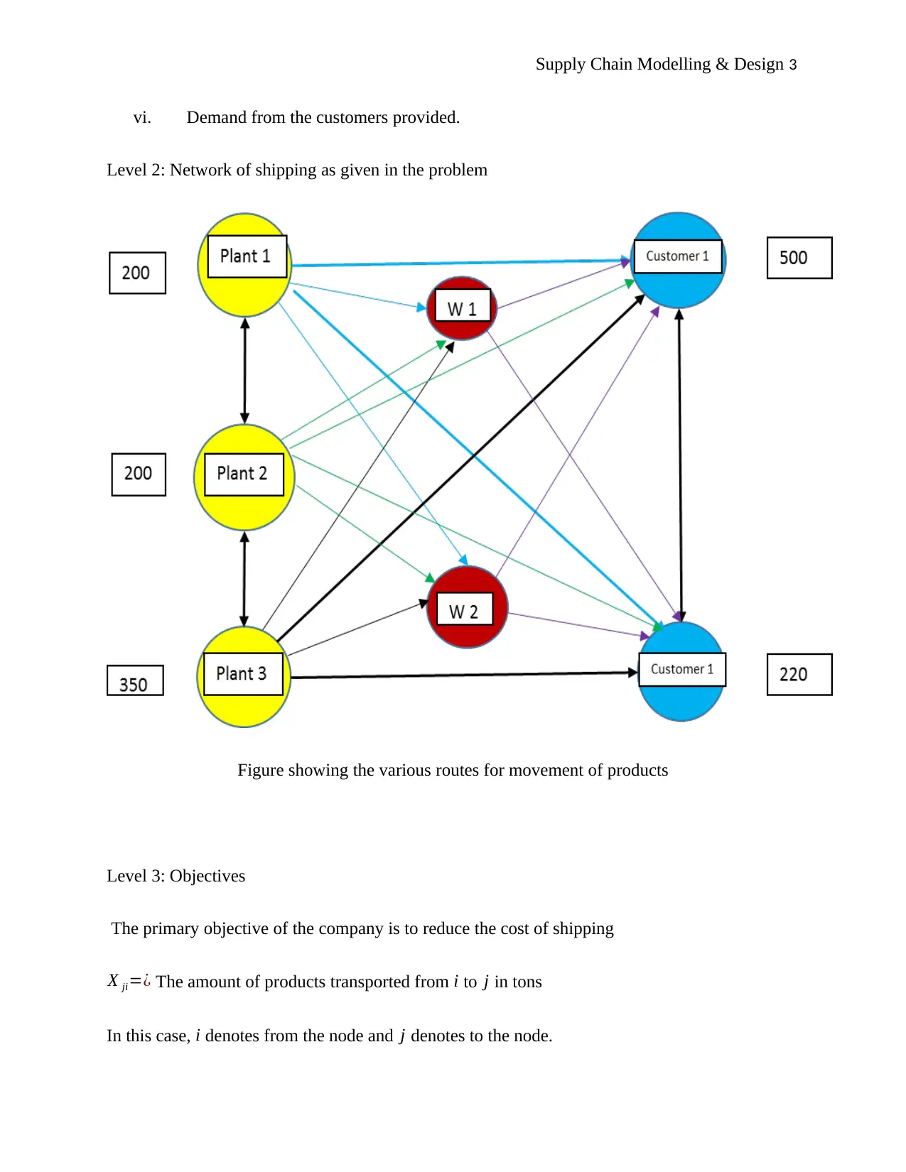
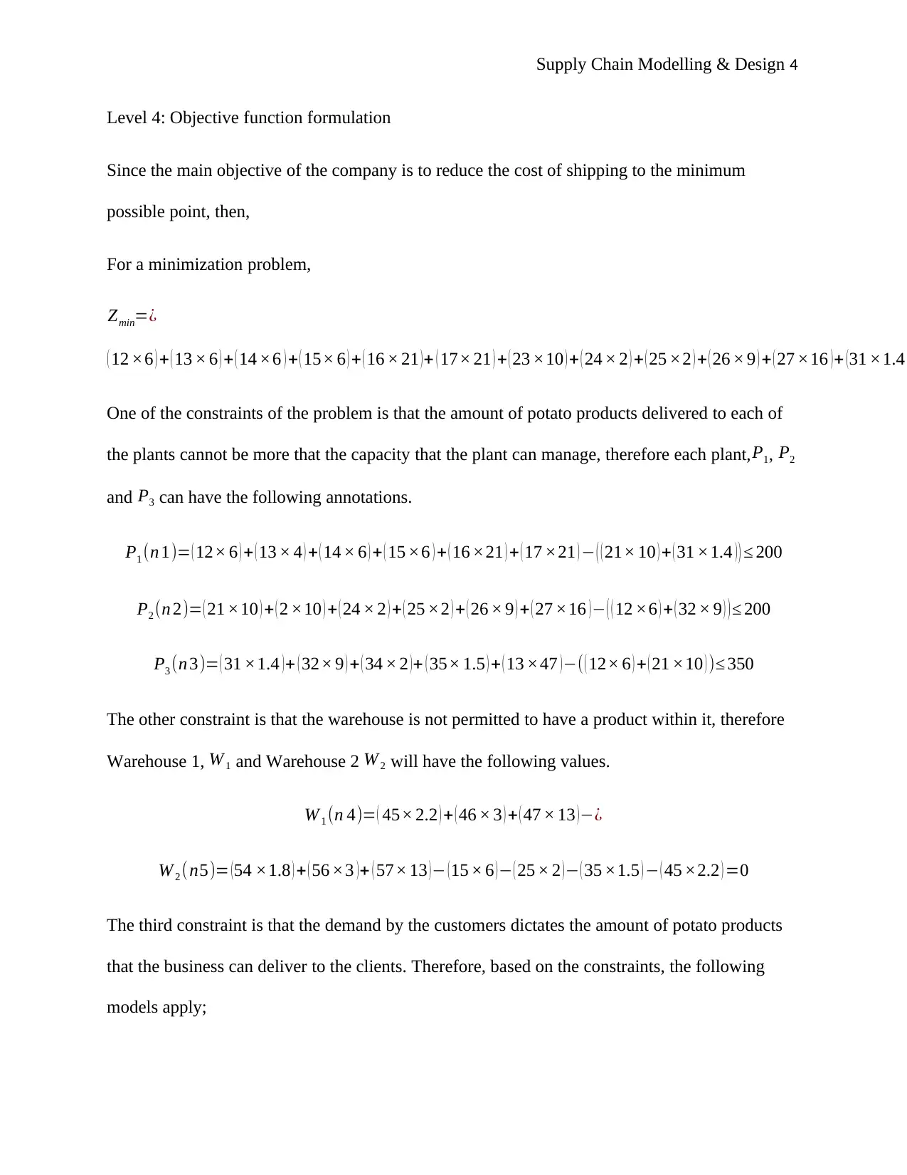
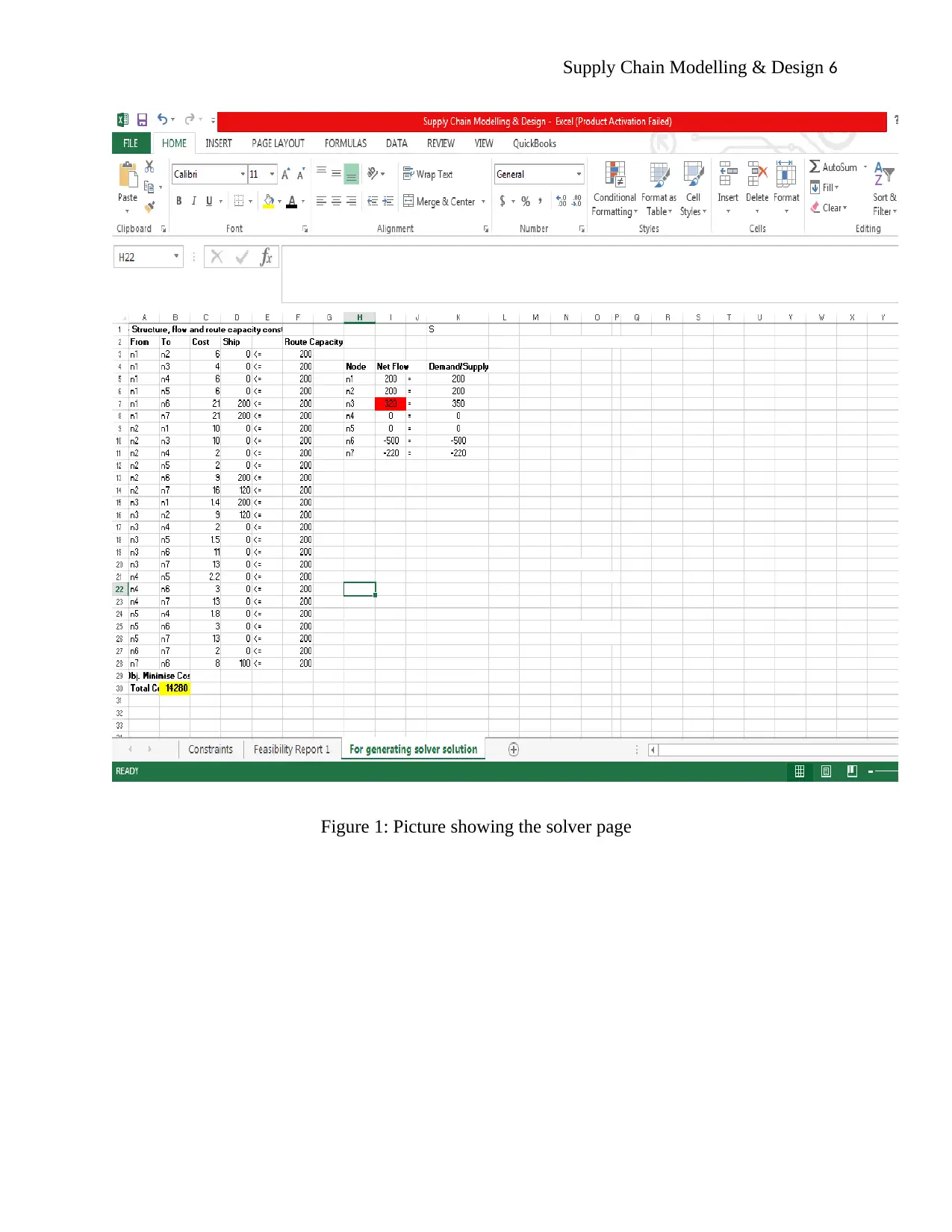
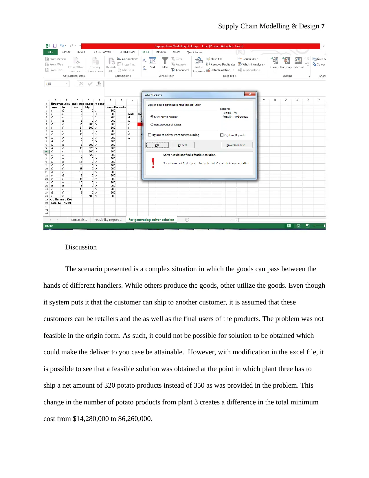
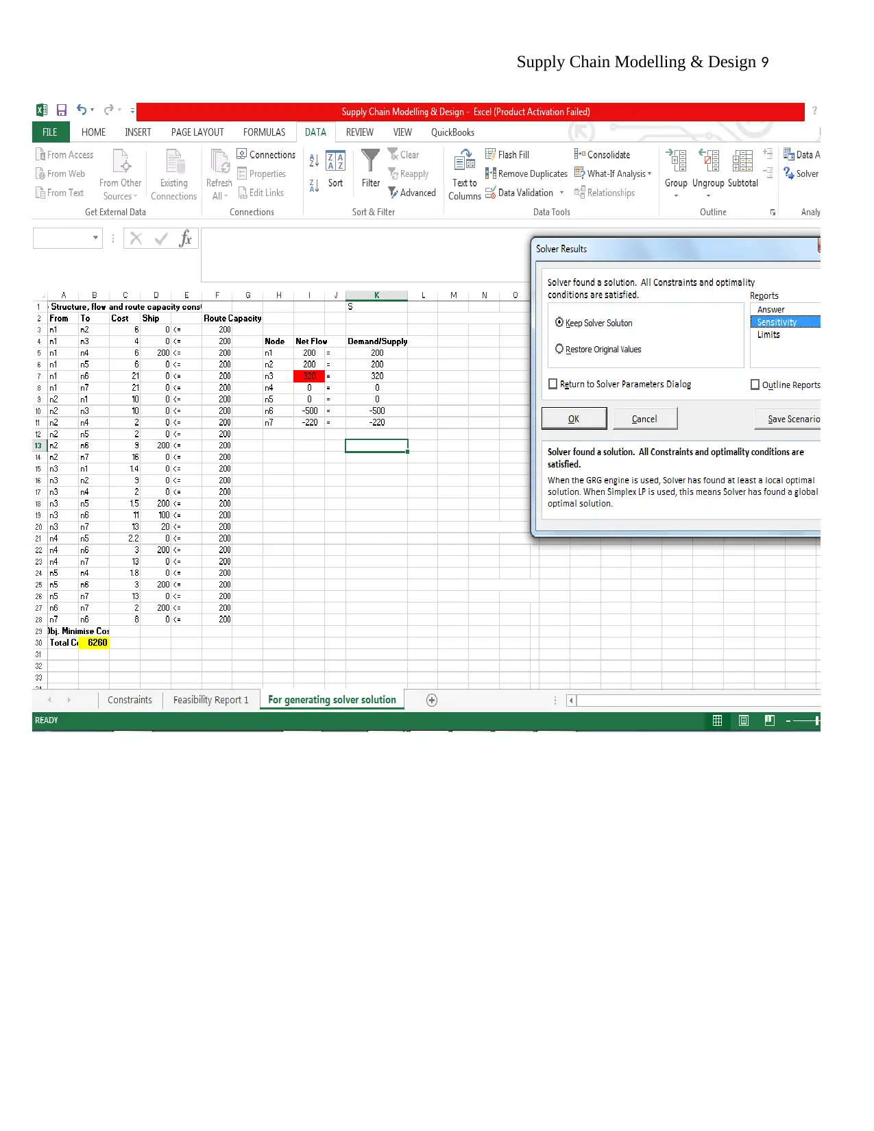
This case study examines a supply chain model for a company producing potato products across three plants, two warehouses, and two customers. The primary objective is to minimize total shipping costs, considering plant capacities and customer demands. The analysis involves formulating the problem, defining decision variables, and establishing objective functions with constraints. A graphical model illustrates the supply chain network, and mathematical models are developed to represent the transportation problem. Excel is used to implement and solve the linear programming model, with the goal of determining the most cost-effective shipping routes. The solution identifies an optimal shipping plan with a minimum cost of $6,260,000, achieved by adjusting plant output. The study also highlights the importance of considering various constraints, such as plant capacity, warehouse limitations, and customer demand, to ensure a feasible and efficient supply chain. The case study provides recommendations for optimizing the supply chain, such as ensuring that the total product supply from plant three is adjusted to 320 units. This is a critical step in achieving cost-effective and efficient supply chain operations.

Supply Chain Modelling & Design 1
SUPPLY CHAIN MODELLING & DESIGN
By
Name
Institution
Professor
City and State
Date
City and State

Supply Chain Modelling & Design 2
Supply Chain Modelling & Design
Introduction
Demand and supply of products is one of the most complex issues in business operations.
Since demand and supply both depend on each other, it is necessary that the suppliers know what
is really demanded in the business. As such, several factors must be considered. Specifically, the
suppliers have to know what costs need to be incurred as they supply the products to the
customers. However, since the intention is for the goods to reach the final users, it calls for the
suppliers to determine the minimum cost possible for such an operation (Brandenburg, et al.,
2014). Mathematical models can be used based on the routes which the goods have to follow to
reach the customers (Beamon, 1998). Excel is also used to change various variables within the
system to attain the minimum possible costs. Transportation problems are used more often in
supply chain management.
This paper shows graphical and mathematical models of a supply chain based on the
situation given. The graphical model shows the visual scenario in the routes and specific points
where the goods have to rest. Each route is associated with its own specific cost, which assists
with the determination of the minimum cost.
Level 1. Analysis of the data provided
i. Fixed cost for operation
ii. Products produced by the company- potatoes
iii. Plant capacity in tonnes each year, for each plant.
iv. Fixed constraint provided
v. Variables for shipping are given

Supply Chain Modelling & Design 3
vi. Demand from the customers provided.
Level 2: Network of shipping as given in the problem
Figure showing the various routes for movement of products
Level 3: Objectives
The primary objective of the company is to reduce the cost of shipping
X ji=¿ The amount of products transported from i to j in tons
In this case, i denotes from the node and j denotes to the node.

Supply Chain Modelling & Design 4
Level 4: Objective function formulation
Since the main objective of the company is to reduce the cost of shipping to the minimum
possible point, then,
For a minimization problem,
Zmin=¿
( 12 ×6 ) + ( 13 × 6 ) + ( 14 ×6 ) + ( 15× 6 ) + ( 16 × 21 ) + ( 17× 21 ) + ( 23 ×10 ) + ( 24 × 2 ) + ( 25 ×2 ) + ( 26 × 9 ) + ( 27 ×16 ) + ( 31 ×1.4
One of the constraints of the problem is that the amount of potato products delivered to each of
the plants cannot be more that the capacity that the plant can manage, therefore each plant, P1, P2
and P3 can have the following annotations.
P1 (n 1)= ( 12× 6 ) + ( 13 × 4 ) + ( 14 × 6 ) + ( 15 ×6 ) + ( 16 ×21 ) + ( 17 ×21 ) − ( ( 21× 10 ) + ( 31 ×1.4 ) ) ≤ 200
P2 (n 2)= ( 21 ×10 ) + ( 2 ×10 ) + ( 24 × 2 ) + ( 25 ×2 ) + ( 26 × 9 ) + ( 27 ×16 ) − ( ( 12 ×6 ) + ( 32 × 9 ) ) ≤ 200
P3 (n 3)= ( 31 ×1.4 ) + ( 32× 9 ) + ( 34 × 2 ) + ( 35× 1.5 ) + ( 13 ×47 ) −( ( 12× 6 ) + ( 21 ×10 ) )≤ 350
The other constraint is that the warehouse is not permitted to have a product within it, therefore
Warehouse 1, W1 and Warehouse 2 W2 will have the following values.
W 1 (n 4)= ( 45× 2.2 ) + ( 46 × 3 ) + ( 47 × 13 ) −¿
W2 (n5)= (54 ×1.8 ) + ( 56 ×3 )+ ( 57× 13 )− (15 × 6 )− ( 25 × 2 )− ( 35 ×1.5 ) − ( 45 ×2.2 ) =0
The third constraint is that the demand by the customers dictates the amount of potato products
that the business can deliver to the clients. Therefore, based on the constraints, the following
models apply;

Supply Chain Modelling & Design 5
C1(n 6)= ( 16 ×12 ) + ( 26 × 9 ) + ( 36 ×11 ) + ( 46× 3 ) + ( 56 ×3 )+ ( 76× 3 )− ( 67× 2 )=500
C2(n 7)= ( 17 ×21 ) + ( 27 ×16 ) + ( 37 ×13 ) + ( 47 ×13 ) + ( 57 ×13 )+ ( 67 ×2 )− (76 × 8 )=220
The fourth constraints is that it is not possible to change the route capacity so that the flow of
good is constrained to less than 200. That is;
Flow of products ≤ 200
The fifth constraint is the impossibility of change in the decision variables, which cannot be less
than zero. This implies that whatever decision is chosenX ji ≥ 0.

Supply Chain Modelling & Design 6
Figure 1: Picture showing the solver page

Supply Chain Modelling & Design 7
Discussion
The scenario presented is a complex situation in which the goods can pass between the
hands of different handlers. While others produce the goods, other utilize the goods. Even though
it system puts it that the customer can ship to another customer, it is assumed that these
customers can be retailers and the as well as the final users of the products. The problem was not
feasible in the origin form. As such, it could not be possible for solution to be obtained which
could make the deliver to you case be attainable. However, with modification in the excel file, it
is possible to see that a feasible solution was obtained at the point in which plant three has to
ship a net amount of 320 potato products instead of 350 as was provided in the problem. This
change in the number of potato products from plant 3 creates a difference in the total minimum
cost from $14,280,000 to $6,260,000.

Supply Chain Modelling & Design 8
The net flow of goods also matches the expected scenario. For instance plant 1, 2 and 3,
represented by nodes 1, node 2 and node 3 are all bring their products into the system. The two
warehouses, however, do not use the products and neither do they bring in more products into the
system. However, the values of the customers are negative. This shows that the customers are
taking the products out of the system.
Recommendation and Conclusion
Based on the linear programming solution obtained from the excel (Liang &
Miikkulainen, 2015), the following recommendations can be made.
1. Plant three supplies an excess of 30 products. As such, the net flow from the plant should
be 320 potato products.
The original supply for plant 3, which was 350 produced infeasible solution in the excel
solver. However, the solver produced a net flow of 320 from plant 3, which when
replaced in the supply column produces a feasible solution.
Conclusion
As a result, the new minimum cost for the shipping is obtained to be $ 6,260,000.

Supply Chain Modelling & Design 9

Supply Chain Modelling & Design
10
References
Beamon, B. M., 1998. Supply chain design and analysis:: Models and methods. International
journal of production economics, 55(3), pp. 281-294.
Brandenburg, M., Govindan, K., Sarkis, J. & Seuring, S., 2014. Quantitative models for
sustainable supply chain management: Developments and directions. European Journal of
Operational Research, 233(2), pp. 299-312.
Liang, J. Z. & Miikkulainen, R., 2015. Evolutionary bilevel optimization for complex control
tasks. s.l., ACM., pp. 871-878.