OMGT2287: Supply Chain Modeling and Design Project Analysis
VerifiedAdded on 2023/06/10
|20
|4407
|280
Project
AI Summary
This document presents a comprehensive solution to a supply chain modeling and design assignment. The solution addresses a case study involving recycling operations across ten sectors and five recycling sites. It utilizes multi-objective linear programming (MOLP) to optimize garbage tonnage maximization and transportation cost minimization, considering site capacities and efficiencies. The assignment explores problem formulation, constraint definition, and the application of Excel Solver to determine optimal solutions. The analysis includes detailed calculations, solver outputs, and interpretations of the results. The document also addresses warehouse location optimization to minimize distances between different locations. The solution provides a complete breakdown of the problem, methodologies, and findings, offering insights into supply chain decision-making techniques and optimization strategies. The project delves into waste management and recycling site efficiency, using MOLP for optimal resource allocation.
Supply Chain Modelling and Design
Paraphrase This Document
Need a fresh take? Get an instant paraphrase of this document with our AI Paraphraser
Decision Making Techniques
Contents
Solution of Problem 1......................................................................................................................2
Sol.1(a).........................................................................................................................................2
Sol.1(b)........................................................................................................................................6
Sol.1(c).........................................................................................................................................7
Solution of problem 2....................................................................................................................10
Solution for Problem 3...................................................................................................................12
Solution for Problem 4...................................................................................................................14
References......................................................................................................................................17
1 | P a g e
Decision Making Techniques
Solution of Problem 1
Sol.1(a)
As per given condition in problem, we have to solve the situation using multi objective linear
programming (MOLP), In order to solve the problem using MOLP first we will solve the
individual objective using solver, from this two-unit objective in which one increasing garbage
capacity and another one is minimising transportation cost. The calculated result set as target for
MOLP and we should provide weighted condition with few more constraints, so that we can
achieve minimax condition of desired result.
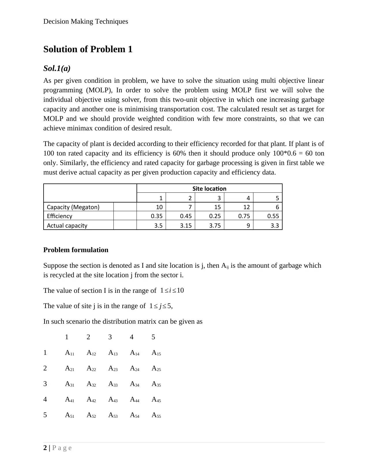
The capacity of plant is decided according to their efficiency recorded for that plant. If plant is of
100 ton rated capacity and its efficiency is 60% then it should produce only 100*0.6 = 60 ton
only. Similarly, the efficiency and rated capacity for garbage processing is given in first table we
must derive actual capacity as per given production capacity and efficiency data.
Site location
1 2 3 4 5
Capacity (Megaton) 10 7 15 12 6
Efficiency 0.35 0.45 0.25 0.75 0.55
Actual capacity 3.5 3.15 3.75 9 3.3
Problem formulation
Suppose the section is denoted as I and site location is j, then Aij is the amount of garbage which
is recycled at the site location j from the sector i.
The value of section I is in the range of 1 ≤i ≤10
The value of site j is in the range of 1 ≤ j≤ 5,
In such scenario the distribution matrix can be given as
1 2 3 4 5
1 A11 A12 A13 A14 A15
2 A21 A22 A23 A24 A25
3 A31 A32 A33 A34 A35
4 A41 A42 A43 A44 A45
5 A51 A52 A53 A54 A55
2 | P a g e
Solution of Problem 1
Sol.1(a)
As per given condition in problem, we have to solve the situation using multi objective linear
programming (MOLP), In order to solve the problem using MOLP first we will solve the
individual objective using solver, from this two-unit objective in which one increasing garbage
capacity and another one is minimising transportation cost. The calculated result set as target for
MOLP and we should provide weighted condition with few more constraints, so that we can
achieve minimax condition of desired result.
The capacity of plant is decided according to their efficiency recorded for that plant. If plant is of
100 ton rated capacity and its efficiency is 60% then it should produce only 100*0.6 = 60 ton
only. Similarly, the efficiency and rated capacity for garbage processing is given in first table we
must derive actual capacity as per given production capacity and efficiency data.
Site location
1 2 3 4 5
Capacity (Megaton) 10 7 15 12 6
Efficiency 0.35 0.45 0.25 0.75 0.55
Actual capacity 3.5 3.15 3.75 9 3.3
Problem formulation
Suppose the section is denoted as I and site location is j, then Aij is the amount of garbage which
is recycled at the site location j from the sector i.
The value of section I is in the range of 1 ≤i ≤10
The value of site j is in the range of 1 ≤ j≤ 5,
In such scenario the distribution matrix can be given as
1 2 3 4 5
1 A11 A12 A13 A14 A15
2 A21 A22 A23 A24 A25
3 A31 A32 A33 A34 A35
4 A41 A42 A43 A44 A45
5 A51 A52 A53 A54 A55
2 | P a g e
⊘ This is a preview!⊘
Do you want full access?
Subscribe today to unlock all pages.
Trusted by 1+ million students worldwide
Decision Making Techniques
6 A61 A62 A63 A64 A65
7 A71 A72 A73 A74 A75
8 A81 A82 A83 A84 A85
9 A91 A92 A93 A94 A95
10 A101 A102 A103 A104 A105
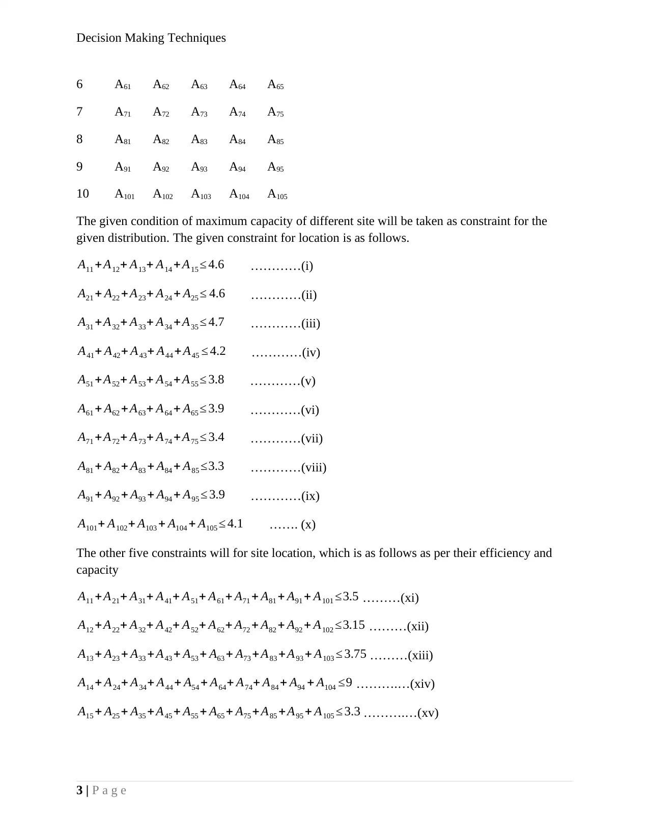
The given condition of maximum capacity of different site will be taken as constraint for the
given distribution. The given constraint for location is as follows.
A11 + A12+ A13+ A14 + A15 ≤ 4.6 …………(i)
A21 + A22 + A23+ A24 + A25 ≤ 4.6 …………(ii)
A31 +A32+ A33+ A34 +A35 ≤ 4.7 …………(iii)
A41+ A42+ A43+ A44 + A45 ≤ 4.2 …………(iv)
A51 + A52+ A53+ A54 + A55 ≤ 3.8 …………(v)
A61 + A62 + A63+ A64 + A65 ≤ 3.9 …………(vi)
A71 +A72+ A73+ A74 +A75 ≤ 3.4 …………(vii)
A81 + A82 + A83 + A84 + A85 ≤3.3 …………(viii)
A91 + A92 + A93 + A94 + A95 ≤ 3.9 …………(ix)
A101+ A102+ A103 + A104 + A105 ≤ 4.1 ……. (x)
The other five constraints will for site location, which is as follows as per their efficiency and
capacity
A11 + A21+ A31+ A41+ A51+ A61+ A71 + A81 + A91 + A101 ≤3.5 ………(xi)
A12 + A22+ A32+ A42+ A52+ A62+ A72 + A82 + A92 + A102 ≤3.15 ………(xii)
A13 + A23 + A33 +A43 + A53 + A63 + A73 + A83 + A93 + A103 ≤ 3.75 ………(xiii)
A14 + A24+ A34+ A44 + A54 + A64+ A74+ A84 + A94 + A104 ≤9 ……….…(xiv)
A15 + A25 + A35 +A45 + A55 + A65 + A75 + A85 + A95 + A105 ≤ 3.3 ……….…(xv)
3 | P a g e
6 A61 A62 A63 A64 A65
7 A71 A72 A73 A74 A75
8 A81 A82 A83 A84 A85
9 A91 A92 A93 A94 A95
10 A101 A102 A103 A104 A105
The given condition of maximum capacity of different site will be taken as constraint for the
given distribution. The given constraint for location is as follows.
A11 + A12+ A13+ A14 + A15 ≤ 4.6 …………(i)
A21 + A22 + A23+ A24 + A25 ≤ 4.6 …………(ii)
A31 +A32+ A33+ A34 +A35 ≤ 4.7 …………(iii)
A41+ A42+ A43+ A44 + A45 ≤ 4.2 …………(iv)
A51 + A52+ A53+ A54 + A55 ≤ 3.8 …………(v)
A61 + A62 + A63+ A64 + A65 ≤ 3.9 …………(vi)
A71 +A72+ A73+ A74 +A75 ≤ 3.4 …………(vii)
A81 + A82 + A83 + A84 + A85 ≤3.3 …………(viii)
A91 + A92 + A93 + A94 + A95 ≤ 3.9 …………(ix)
A101+ A102+ A103 + A104 + A105 ≤ 4.1 ……. (x)
The other five constraints will for site location, which is as follows as per their efficiency and
capacity
A11 + A21+ A31+ A41+ A51+ A61+ A71 + A81 + A91 + A101 ≤3.5 ………(xi)
A12 + A22+ A32+ A42+ A52+ A62+ A72 + A82 + A92 + A102 ≤3.15 ………(xii)
A13 + A23 + A33 +A43 + A53 + A63 + A73 + A83 + A93 + A103 ≤ 3.75 ………(xiii)
A14 + A24+ A34+ A44 + A54 + A64+ A74+ A84 + A94 + A104 ≤9 ……….…(xiv)
A15 + A25 + A35 +A45 + A55 + A65 + A75 + A85 + A95 + A105 ≤ 3.3 ……….…(xv)
3 | P a g e
Paraphrase This Document
Need a fresh take? Get an instant paraphrase of this document with our AI Paraphraser
Decision Making Techniques
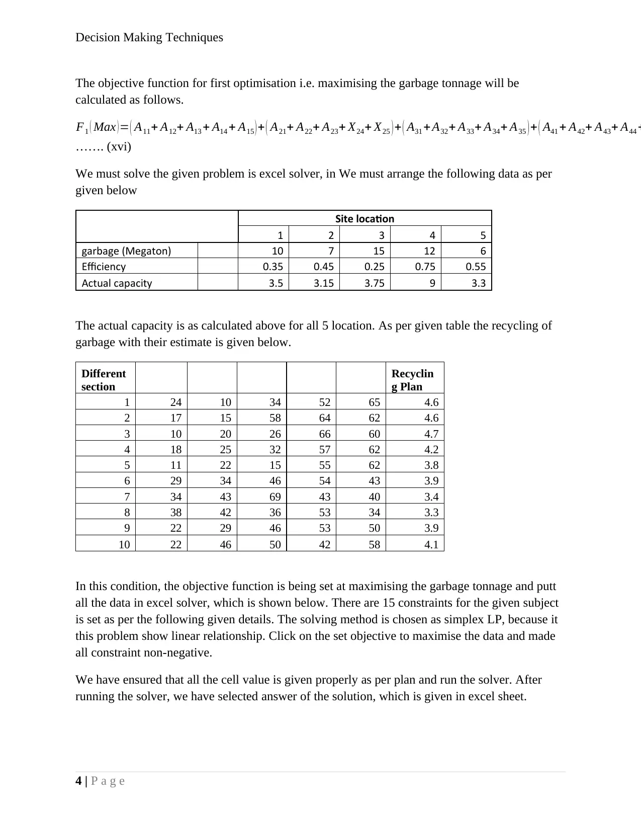
The objective function for first optimisation i.e. maximising the garbage tonnage will be
calculated as follows.
F1 ( Max )= ( A11+ A12+ A13 + A14 + A15 ) + ( A21+ A22+ A23+ X24+ X25 ) + ( A31 + A32+ A33+ A34+ A35 )+ ( A41 + A42+ A43+ A44 +
……. (xvi)
We must solve the given problem is excel solver, in We must arrange the following data as per
given below
Site location
1 2 3 4 5
garbage (Megaton) 10 7 15 12 6
Efficiency 0.35 0.45 0.25 0.75 0.55
Actual capacity 3.5 3.15 3.75 9 3.3
The actual capacity is as calculated above for all 5 location. As per given table the recycling of
garbage with their estimate is given below.
Different
section
Recyclin
g Plan
1 24 10 34 52 65 4.6
2 17 15 58 64 62 4.6
3 10 20 26 66 60 4.7
4 18 25 32 57 62 4.2
5 11 22 15 55 62 3.8
6 29 34 46 54 43 3.9
7 34 43 69 43 40 3.4
8 38 42 36 53 34 3.3
9 22 29 46 53 50 3.9
10 22 46 50 42 58 4.1
In this condition, the objective function is being set at maximising the garbage tonnage and putt
all the data in excel solver, which is shown below. There are 15 constraints for the given subject
is set as per the following given details. The solving method is chosen as simplex LP, because it
this problem show linear relationship. Click on the set objective to maximise the data and made
all constraint non-negative.
We have ensured that all the cell value is given properly as per plan and run the solver. After
running the solver, we have selected answer of the solution, which is given in excel sheet.
4 | P a g e

Decision Making Techniques
After running the solver, the maximum value of garbage recycling occurred is 22.7 megaton. The
result obtained from running the solver illustrates that, the sector number. The capacity is
reached at its optimum level without taking the section 7, 8 ,9, and 10. This show that, the
capacity of recycling site is very low as compared to sum of garbage of 10 sector. We have to
either increase the efficiency of given recycling site or increase the recycling plant for given
capacity of different sector.
5 | P a g e
⊘ This is a preview!⊘
Do you want full access?
Subscribe today to unlock all pages.
Trusted by 1+ million students worldwide
Decision Making Techniques
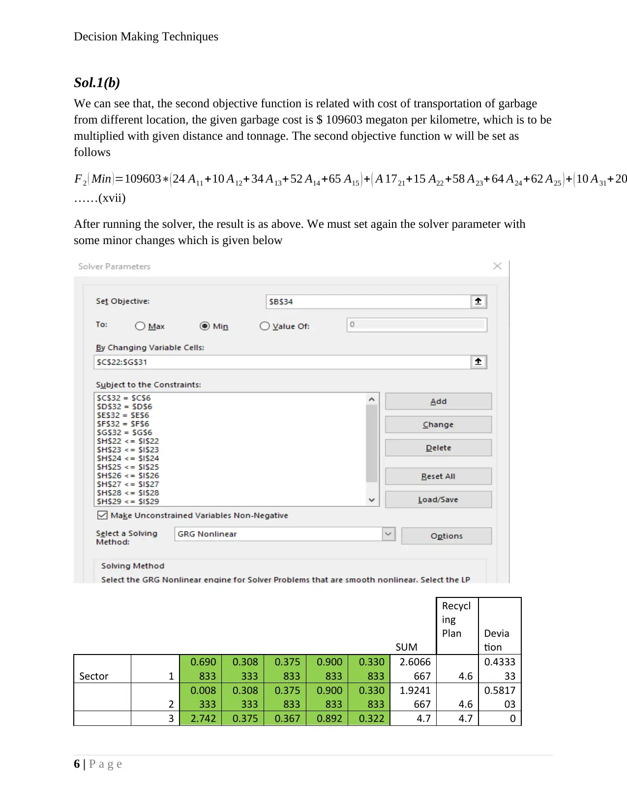
Sol.1(b)
We can see that, the second objective function is related with cost of transportation of garbage
from different location, the given garbage cost is $ 109603 megaton per kilometre, which is to be
multiplied with given distance and tonnage. The second objective function w will be set as
follows
F2 ( Min )=109603∗( 24 A11 +10 A12+ 34 A13+ 52 A14 +65 A15 ) + ( A 1721+15 A22 +58 A23+ 64 A24 +62 A25 ) + ( 10 A31+20
……(xvii)
After running the solver, the result is as above. We must set again the solver parameter with
some minor changes which is given below
SUM
Recycl
ing
Plan Devia
tion
Sector 1
0.690
833
0.308
333
0.375
833
0.900
833
0.330
833
2.6066
667 4.6
0.4333
33
2
0.008
333
0.308
333
0.375
833
0.900
833
0.330
833
1.9241
667 4.6
0.5817
03
3 2.742 0.375 0.367 0.892 0.322 4.7 4.7 0
6 | P a g e
Paraphrase This Document
Need a fresh take? Get an instant paraphrase of this document with our AI Paraphraser
Decision Making Techniques
5 5 5 5
4
0.008
333
0.308
333
0.375
833
0.900
833
0.330
833
1.9241
667 4.2
0.5418
65
5
0.008
333
0.308
333
0.375
833
0.900
833
0.330
833
1.9241
667 3.8
0.4936
4
6
0.008
333
0.308
333
0.375
833
0.900
833
0.330
833
1.9241
667 3.9
0.5066
24
7
0.008
333
0.308
333
0.375
833
0.900
833
0.330
833
1.9241
667 3.4
0.4340
69
8
0.008
333
0.308
333
0.375
833
0.900
833
0.330
833
1.9241
667 3.3
0.4169
19
9
0.008
333
0.308
333
0.375
833
0.900
833
0.330
833
1.9241
667 3.9
0.5066
24
10
0.008
333
0.308
333
0.375
833
0.900
833
0.330
833
1.9241
667 4.1
0.5306
91
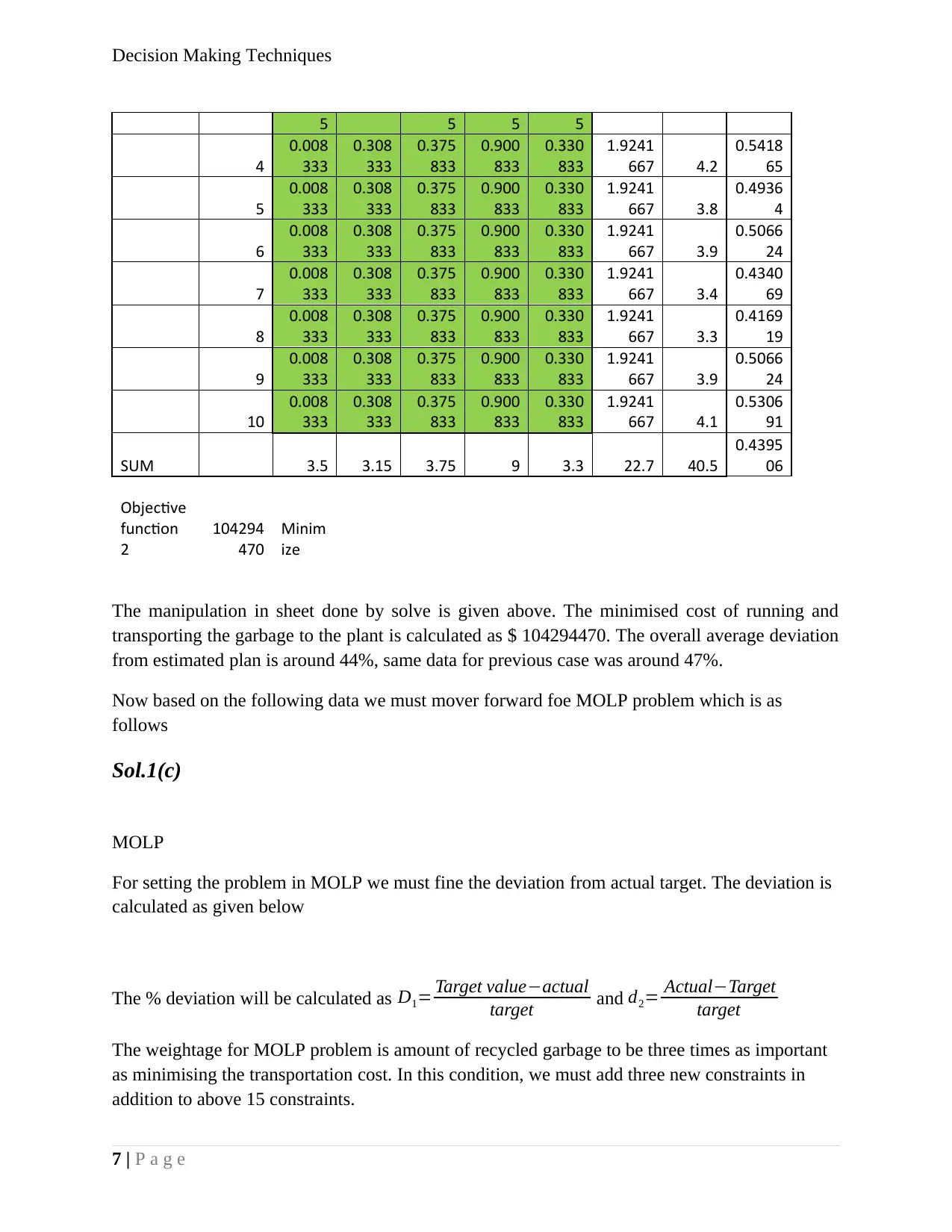
SUM 3.5 3.15 3.75 9 3.3 22.7 40.5
0.4395
06
Objective
function
2
104294
470
Minim
ize
The manipulation in sheet done by solve is given above. The minimised cost of running and
transporting the garbage to the plant is calculated as $ 104294470. The overall average deviation
from estimated plan is around 44%, same data for previous case was around 47%.
Now based on the following data we must mover forward foe MOLP problem which is as
follows
Sol.1(c)
MOLP
For setting the problem in MOLP we must fine the deviation from actual target. The deviation is
calculated as given below
The % deviation will be calculated as D1= Target value−actual
target and d2= Actual−Target
target
The weightage for MOLP problem is amount of recycled garbage to be three times as important
as minimising the transportation cost. In this condition, we must add three new constraints in
addition to above 15 constraints.
7 | P a g e
5 5 5 5
4
0.008
333
0.308
333
0.375
833
0.900
833
0.330
833
1.9241
667 4.2
0.5418
65
5
0.008
333
0.308
333
0.375
833
0.900
833
0.330
833
1.9241
667 3.8
0.4936
4
6
0.008
333
0.308
333
0.375
833
0.900
833
0.330
833
1.9241
667 3.9
0.5066
24
7
0.008
333
0.308
333
0.375
833
0.900
833
0.330
833
1.9241
667 3.4
0.4340
69
8
0.008
333
0.308
333
0.375
833
0.900
833
0.330
833
1.9241
667 3.3
0.4169
19
9
0.008
333
0.308
333
0.375
833
0.900
833
0.330
833
1.9241
667 3.9
0.5066
24
10
0.008
333
0.308
333
0.375
833
0.900
833
0.330
833
1.9241
667 4.1
0.5306
91
SUM 3.5 3.15 3.75 9 3.3 22.7 40.5
0.4395
06
Objective
function
2
104294
470
Minim
ize
The manipulation in sheet done by solve is given above. The minimised cost of running and
transporting the garbage to the plant is calculated as $ 104294470. The overall average deviation
from estimated plan is around 44%, same data for previous case was around 47%.
Now based on the following data we must mover forward foe MOLP problem which is as
follows
Sol.1(c)
MOLP
For setting the problem in MOLP we must fine the deviation from actual target. The deviation is
calculated as given below
The % deviation will be calculated as D1= Target value−actual
target and d2= Actual−Target
target
The weightage for MOLP problem is amount of recycled garbage to be three times as important
as minimising the transportation cost. In this condition, we must add three new constraints in
addition to above 15 constraints.
7 | P a g e
Decision Making Techniques
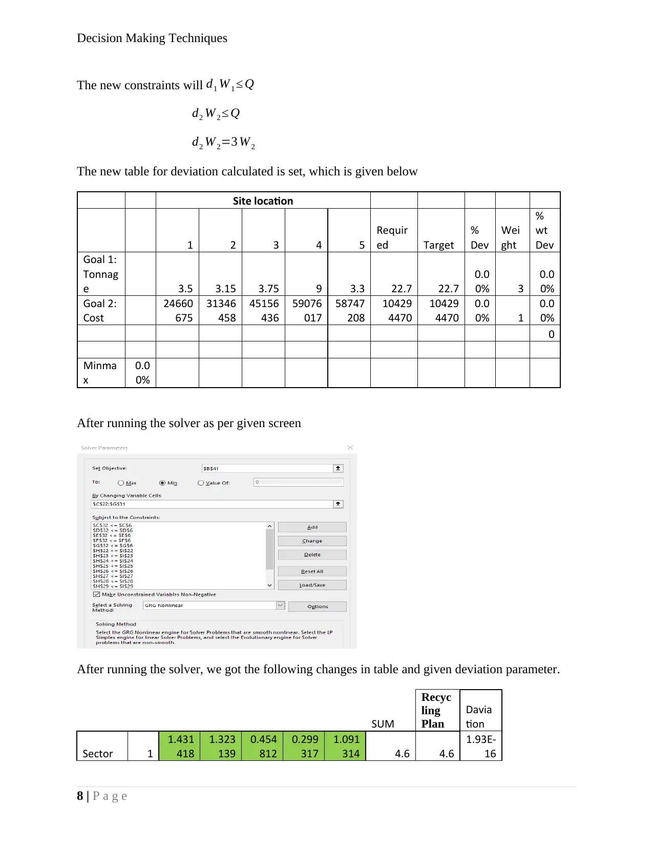
The new constraints will d1 W 1 ≤ Q
d2 W2 ≤ Q
d2 W2=3 W 2
The new table for deviation calculated is set, which is given below
Site location
1 2 3 4 5
Requir
ed Target
%
Dev
Wei
ght
%
wt
Dev
Goal 1:
Tonnag
e 3.5 3.15 3.75 9 3.3 22.7 22.7
0.0
0% 3
0.0
0%
Goal 2:
Cost
24660
675
31346
458
45156
436
59076
017
58747
208
10429
4470
10429
4470
0.0
0% 1
0.0
0%
0
Minma
x
0.0
0%
After running the solver as per given screen
After running the solver, we got the following changes in table and given deviation parameter.
SUM
Recyc
ling
Plan
Davia
tion
Sector 1
1.431
418
1.323
139
0.454
812
0.299
317
1.091
314 4.6 4.6
1.93E-
16
8 | P a g e
⊘ This is a preview!⊘
Do you want full access?
Subscribe today to unlock all pages.
Trusted by 1+ million students worldwide

Decision Making Techniques
2
0.448
159
0.209
79
0.251
432
0.896
66
0.294
085
2.1001
2444 4.6
0.543
451
3
0.265
121
0.942
066
0.510
643
0.887
122
0.501
25
3.1062
0062 4.7
0.339
106
4
0.410
376
0.152
992
0.445
298
1.111
549
0.391
721
2.5119
3553 4.2
0.401
92
5
0.360
94
0.175
161
0.711
868
1.036
708
0.391
721
2.6763
9808 3.8
0.295
685
6
0.209
151
0.077
886
0.012
73
1.223
593
0.006
104
1.5294
6406 3.9
0.607
83
7
0.060
629
0.007
72
0.657
372
0.706
848
0.032
456
1.4650
2475 3.4
0.569
11
8 0 0
0.527
407
0.898
235
0.302
792
1.7284
3391 3.3
0.476
232
9
0.156
556
0.226
407
0.012
73
1.015
131
0.070
101
1.4809
2556 3.9
0.620
275
10
0.157
652
0.034
84
0.165
71
0.924
837
0.218
454
1.5014
9305 4.1
0.633
782
SUM 3.5 3.15 3.75 9 3.3 22.7 40.5
0.439
506
Site location
1 2 3 4 5
Requir
ed Target
%
Dev
Wei
ght
%
wt
Dev
Goal 1:
Tonnag
e 3.5 3.15 3.75 9 3.3 22.7 22.7
0.0
0% 3
0.0
0%
Goal 2:
Cost
24660
675
31346
458
45156
436
59076
017
58747
208
104294
470
104294
470
0.0
0% 1
0.0
0%
0
Minmax
0.0
0%
The calculated parameter by MOLP solver suggests that, the optimisation done in previous
condition individually has the most optimum solution for given condition and the is not change
in parameter after giving the weightage and deviation condition. So, the suggestion given for first
objective function is still viable for this condition also. Similarly, the cost objective is also
remain unchanged due to plant capacity problem.
9 | P a g e
Paraphrase This Document
Need a fresh take? Get an instant paraphrase of this document with our AI Paraphraser
Decision Making Techniques
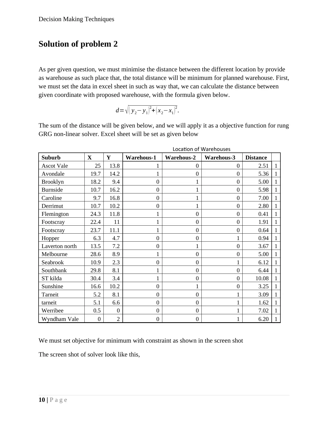
Solution of problem 2
As per given question, we must minimise the distance between the different location by provide
as warehouse as such place that, the total distance will be minimum for planned warehouse. First,
we must set the data in excel sheet in such as way that, we can calculate the distance between
given coordinate with proposed warehouse, with the formula given below.
d= √ ( y2− y1 ) 2+ ( x2−x1 ) 2.
The sum of the distance will be given below, and we will apply it as a objective function for rung
GRG non-linear solver. Excel sheet will be set as given below
Location of Warehouses
Suburb X Y Warehous-1 Warehous-2 Warehous-3 Distance
Ascot Vale 25 13.8 1 0 0 2.51 1
Avondale 19.7 14.2 1 0 0 5.36 1
Brooklyn 18.2 9.4 0 1 0 5.00 1
Burnside 10.7 16.2 0 1 0 5.98 1
Caroline 9.7 16.8 0 1 0 7.00 1
Derrimut 10.7 10.2 0 1 0 2.80 1
Flemington 24.3 11.8 1 0 0 0.41 1
Footscray 22.4 11 1 0 0 1.91 1
Footscray 23.7 11.1 1 0 0 0.64 1
Hopper 6.3 4.7 0 0 1 0.94 1
Laverton north 13.5 7.2 0 1 0 3.67 1
Melbourne 28.6 8.9 1 0 0 5.00 1
Seabrook 10.9 2.3 0 0 1 6.12 1
Southbank 29.8 8.1 1 0 0 6.44 1
ST kilda 30.4 3.4 1 0 0 10.08 1
Sunshine 16.6 10.2 0 1 0 3.25 1
Tarneit 5.2 8.1 0 0 1 3.09 1
tarneit 5.1 6.6 0 0 1 1.62 1
Werribee 0.5 0 0 0 1 7.02 1
Wyndham Vale 0 2 0 0 1 6.20 1
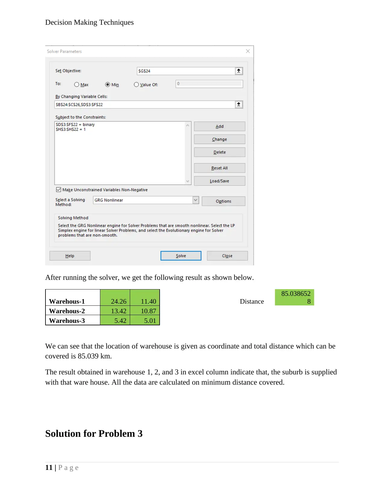
We must set objective for minimum with constraint as shown in the screen shot
The screen shot of solver look like this,
10 | P a g e
Solution of problem 2
As per given question, we must minimise the distance between the different location by provide
as warehouse as such place that, the total distance will be minimum for planned warehouse. First,
we must set the data in excel sheet in such as way that, we can calculate the distance between
given coordinate with proposed warehouse, with the formula given below.
d= √ ( y2− y1 ) 2+ ( x2−x1 ) 2.
The sum of the distance will be given below, and we will apply it as a objective function for rung
GRG non-linear solver. Excel sheet will be set as given below
Location of Warehouses
Suburb X Y Warehous-1 Warehous-2 Warehous-3 Distance
Ascot Vale 25 13.8 1 0 0 2.51 1
Avondale 19.7 14.2 1 0 0 5.36 1
Brooklyn 18.2 9.4 0 1 0 5.00 1
Burnside 10.7 16.2 0 1 0 5.98 1
Caroline 9.7 16.8 0 1 0 7.00 1
Derrimut 10.7 10.2 0 1 0 2.80 1
Flemington 24.3 11.8 1 0 0 0.41 1
Footscray 22.4 11 1 0 0 1.91 1
Footscray 23.7 11.1 1 0 0 0.64 1
Hopper 6.3 4.7 0 0 1 0.94 1
Laverton north 13.5 7.2 0 1 0 3.67 1
Melbourne 28.6 8.9 1 0 0 5.00 1
Seabrook 10.9 2.3 0 0 1 6.12 1
Southbank 29.8 8.1 1 0 0 6.44 1
ST kilda 30.4 3.4 1 0 0 10.08 1
Sunshine 16.6 10.2 0 1 0 3.25 1
Tarneit 5.2 8.1 0 0 1 3.09 1
tarneit 5.1 6.6 0 0 1 1.62 1
Werribee 0.5 0 0 0 1 7.02 1
Wyndham Vale 0 2 0 0 1 6.20 1
We must set objective for minimum with constraint as shown in the screen shot
The screen shot of solver look like this,
10 | P a g e
Decision Making Techniques
After running the solver, we get the following result as shown below.
Warehous-1 24.26 11.40 Distance
85.038652
8
Warehous-2 13.42 10.87
Warehous-3 5.42 5.01
We can see that the location of warehouse is given as coordinate and total distance which can be
covered is 85.039 km.
The result obtained in warehouse 1, 2, and 3 in excel column indicate that, the suburb is supplied
with that ware house. All the data are calculated on minimum distance covered.
Solution for Problem 3
11 | P a g e
⊘ This is a preview!⊘
Do you want full access?
Subscribe today to unlock all pages.
Trusted by 1+ million students worldwide
1 out of 20

Your All-in-One AI-Powered Toolkit for Academic Success.
+13062052269
info@desklib.com
Available 24*7 on WhatsApp / Email
![[object Object]](/_next/static/media/star-bottom.7253800d.svg)
Unlock your academic potential
Copyright © 2020–2026 A2Z Services. All Rights Reserved. Developed and managed by ZUCOL.