Supply Chain Operations Management Report: Case Studies and Analysis

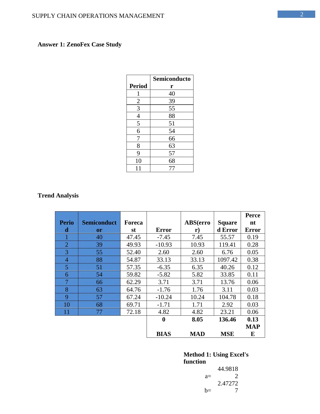
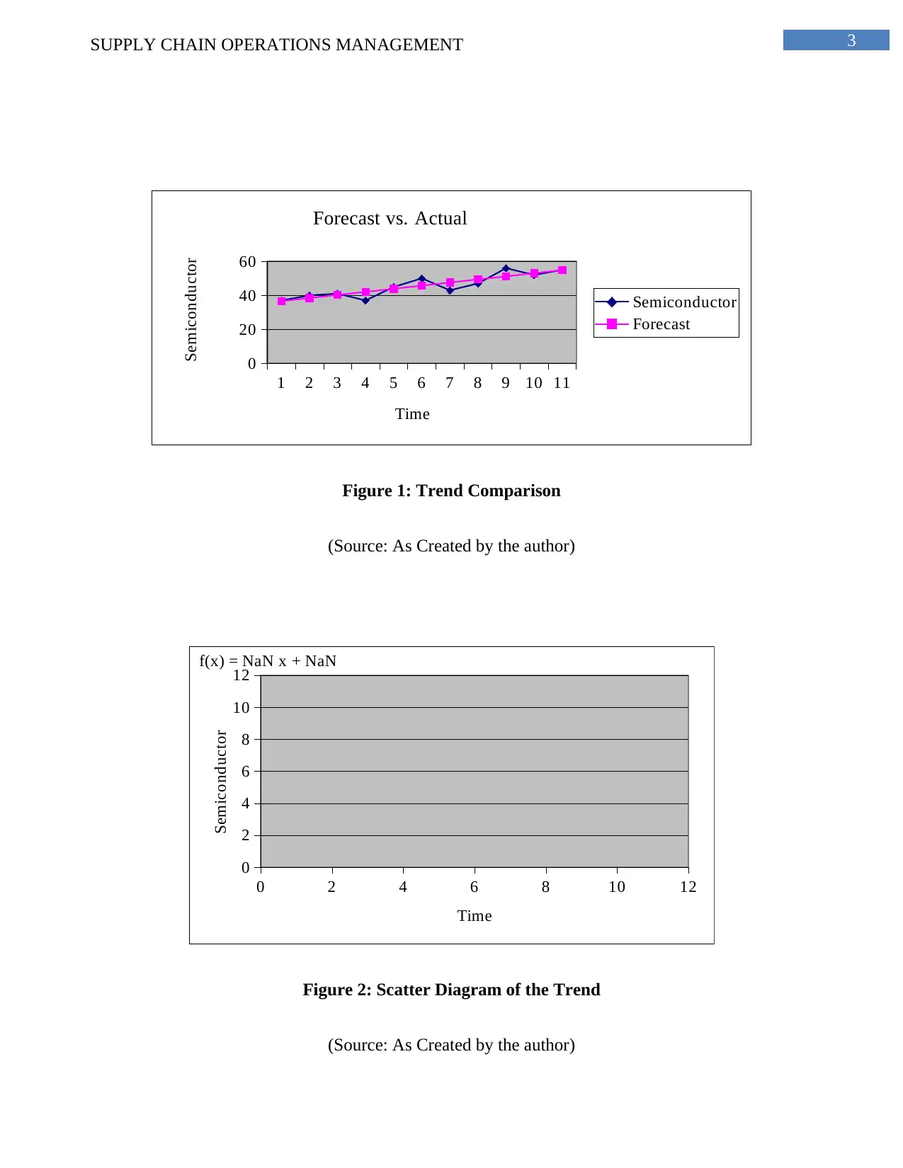
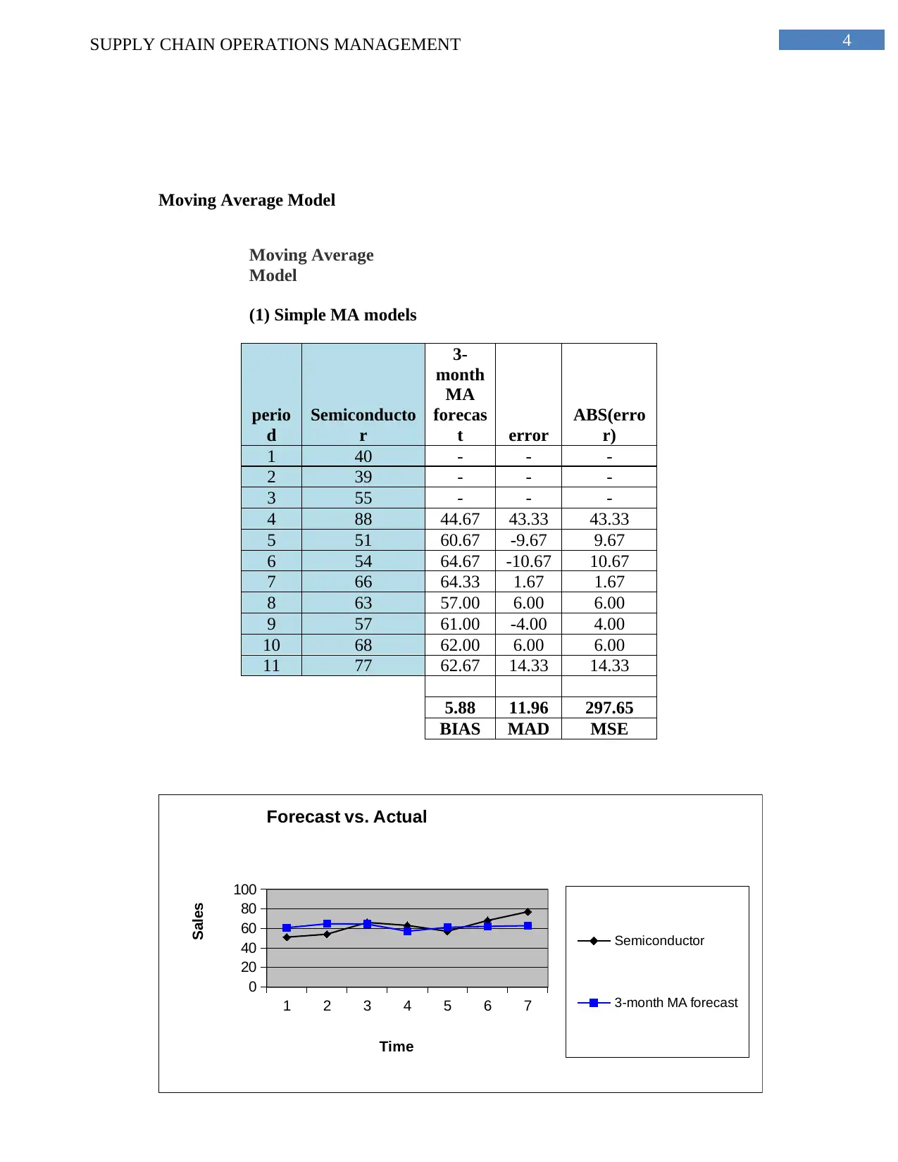
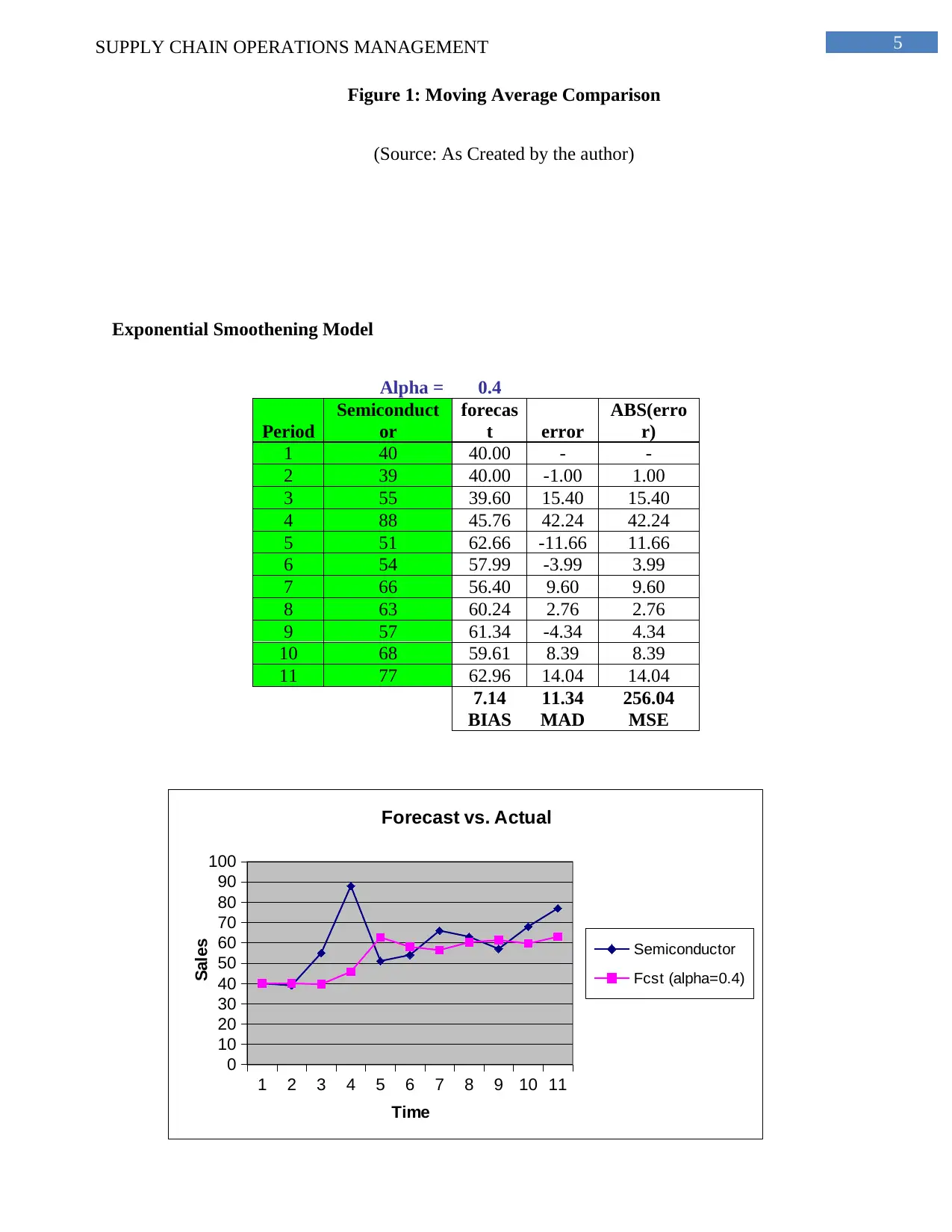
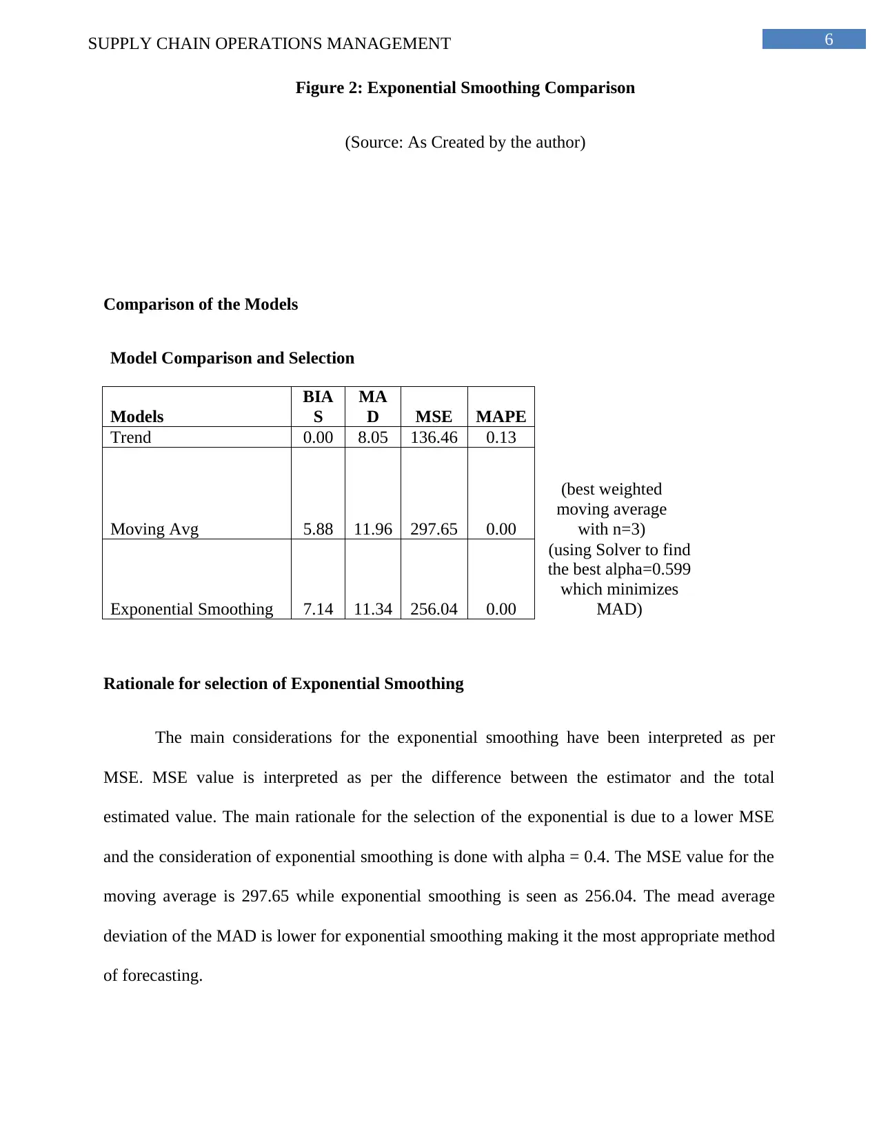
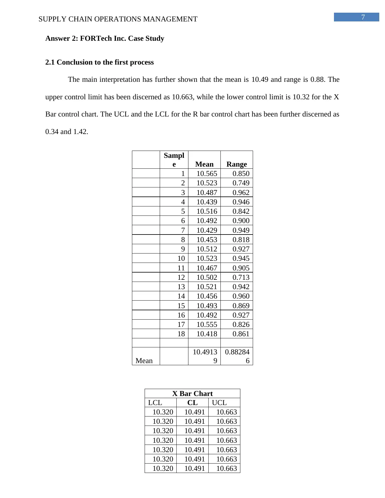
This report delves into the core concepts of supply chain operations management through a detailed analysis of two case studies, ZenoFex and FORTech Inc. The ZenoFex case study explores various forecasting models, including trend analysis, moving average models, and exponential smoothing, comparing their performance using metrics such as BIAS, MAD, MSE, and MAPE to determine the most suitable model. The FORTech Inc. case study focuses on process capability analysis, utilizing X Bar and R Bar control charts to assess process stability and identify areas for improvement. The report computes the process capability index for two datasets, comparing the results and discussing the implications of sample size and data distribution on the overall process performance. The analysis provides insights into the practical application of statistical concepts in supply chain management, highlighting the importance of accurate forecasting and process control for optimizing operational efficiency.

Running head: SUPPLY CHAIN OPERATIONS MANAGEMENT
Supply Chain Operations Management
Name of the Student
Name of the University
Author’s Note

1SUPPLY CHAIN OPERATIONS MANAGEMENT
Table of Contents
Answer 1: ZenoFex Case Study......................................................................................................2
Answer 2: FORTech Inc. Case Study..............................................................................................6
2.1 Conclusion to the first process..............................................................................................6
2.2 Observations in the second process.....................................................................................10
2.3 Computation of the potential process capability using the second data set........................10
2.4 Revealing of the small samples...........................................................................................14
References......................................................................................................................................15

2SUPPLY CHAIN OPERATIONS MANAGEMENT
Answer 1: ZenoFex Case Study
Period
Semiconducto
r
1 40
2 39
3 55
4 88
5 51
6 54
7 66
8 63
9 57
10 68
11 77
Trend Analysis
Perio
d
Semiconduct
or
Foreca
st Error
ABS(erro
r)
Square
d Error
Perce
nt
Error
1 40 47.45 -7.45 7.45 55.57 0.19
2 39 49.93 -10.93 10.93 119.41 0.28
3 55 52.40 2.60 2.60 6.76 0.05
4 88 54.87 33.13 33.13 1097.42 0.38
5 51 57.35 -6.35 6.35 40.26 0.12
6 54 59.82 -5.82 5.82 33.85 0.11
7 66 62.29 3.71 3.71 13.76 0.06
8 63 64.76 -1.76 1.76 3.11 0.03
9 57 67.24 -10.24 10.24 104.78 0.18
10 68 69.71 -1.71 1.71 2.92 0.03
11 77 72.18 4.82 4.82 23.21 0.06
0 8.05 136.46 0.13
BIAS MAD MSE
MAP
E
Method 1: Using Excel's
function
a=
44.9818
2
b=
2.47272
7

3SUPPLY CHAIN OPERATIONS MANAGEMENT
1 2 3 4 5 6 7 8 9 10 11
0
20
40
60
Forecast vs. Actual
Semiconductor
Forecast
Time
Semiconductor
Figure 1: Trend Comparison
(Source: As Created by the author)
0 2 4 6 8 10 12
0
2
4
6
8
10
12
f(x) = NaN x + NaN
Time
Semiconductor
Figure 2: Scatter Diagram of the Trend
(Source: As Created by the author)

4SUPPLY CHAIN OPERATIONS MANAGEMENT
Moving Average Model
Moving Average
Model
(1) Simple MA models
perio
d
Semiconducto
r
3-
month
MA
forecas
t error
ABS(erro
r)
1 40 - - -
2 39 - - -
3 55 - - -
4 88 44.67 43.33 43.33
5 51 60.67 -9.67 9.67
6 54 64.67 -10.67 10.67
7 66 64.33 1.67 1.67
8 63 57.00 6.00 6.00
9 57 61.00 -4.00 4.00
10 68 62.00 6.00 6.00
11 77 62.67 14.33 14.33
5.88 11.96 297.65
BIAS MAD MSE
1 2 3 4 5 6 7
0
20
40
60
80
100
Forecast vs. Actual
Semiconductor
3-month MA forecast
Time
Sales

5SUPPLY CHAIN OPERATIONS MANAGEMENT
Figure 1: Moving Average Comparison
(Source: As Created by the author)
Exponential Smoothening Model
Alpha = 0.4
Period
Semiconduct
or
forecas
t error
ABS(erro
r)
1 40 40.00 - -
2 39 40.00 -1.00 1.00
3 55 39.60 15.40 15.40
4 88 45.76 42.24 42.24
5 51 62.66 -11.66 11.66
6 54 57.99 -3.99 3.99
7 66 56.40 9.60 9.60
8 63 60.24 2.76 2.76
9 57 61.34 -4.34 4.34
10 68 59.61 8.39 8.39
11 77 62.96 14.04 14.04
7.14 11.34 256.04
BIAS MAD MSE
1 2 3 4 5 6 7 8 9 10 11
0
10
20
30
40
50
60
70
80
90
100
Forecast vs. Actual
Semiconductor
Fcst (alpha=0.4)
Time
Sales

6SUPPLY CHAIN OPERATIONS MANAGEMENT
Figure 2: Exponential Smoothing Comparison
(Source: As Created by the author)
Comparison of the Models
Model Comparison and Selection
Models
BIA
S
MA
D MSE MAPE
Trend 0.00 8.05 136.46 0.13
Moving Avg 5.88 11.96 297.65 0.00
(best weighted
moving average
with n=3)
Exponential Smoothing 7.14 11.34 256.04 0.00
(using Solver to find
the best alpha=0.599
which minimizes
MAD)
Rationale for selection of Exponential Smoothing
The main considerations for the exponential smoothing have been interpreted as per
MSE. MSE value is interpreted as per the difference between the estimator and the total
estimated value. The main rationale for the selection of the exponential is due to a lower MSE
and the consideration of exponential smoothing is done with alpha = 0.4. The MSE value for the
moving average is 297.65 while exponential smoothing is seen as 256.04. The mead average
deviation of the MAD is lower for exponential smoothing making it the most appropriate method
of forecasting.

7SUPPLY CHAIN OPERATIONS MANAGEMENT
Answer 2: FORTech Inc. Case Study
2.1 Conclusion to the first process
The main interpretation has further shown that the mean is 10.49 and range is 0.88. The
upper control limit has been discerned as 10.663, while the lower control limit is 10.32 for the X
Bar control chart. The UCL and the LCL for the R bar control chart has been further discerned as
0.34 and 1.42.
Sampl
e Mean Range
1 10.565 0.850
2 10.523 0.749
3 10.487 0.962
4 10.439 0.946
5 10.516 0.842
6 10.492 0.900
7 10.429 0.949
8 10.453 0.818
9 10.512 0.927
10 10.523 0.945
11 10.467 0.905
12 10.502 0.713
13 10.521 0.942
14 10.456 0.960
15 10.493 0.869
16 10.492 0.927
17 10.555 0.826
18 10.418 0.861
Mean
10.4913
9
0.88284
6
X Bar Chart
LCL CL UCL
10.320 10.491 10.663
10.320 10.491 10.663
10.320 10.491 10.663
10.320 10.491 10.663
10.320 10.491 10.663
10.320 10.491 10.663
10.320 10.491 10.663

8SUPPLY CHAIN OPERATIONS MANAGEMENT
10.320 10.491 10.663
10.320 10.491 10.663
10.320 10.491 10.663
10.320 10.491 10.663
10.320 10.491 10.663
10.320 10.491 10.663
10.320 10.491 10.663
10.320 10.491 10.663
10.320 10.491 10.663
10.320 10.491 10.663
10.320 10.491 10.663
R Bar Chart
LCL CL UCL
0.3452 0.883 1.420
0.3452 0.883 1.420
0.3452 0.883 1.420
0.3452 0.883 1.420
0.3452 0.883 1.420
0.3452 0.883 1.420
0.3452 0.883 1.420
0.3452 0.883 1.420
0.3452 0.883 1.420
0.3452 0.883 1.420
0.3452 0.883 1.420
0.3452 0.883 1.420
0.3452 0.883 1.420
0.3452 0.883 1.420
0.3452 0.883 1.420
0.3452 0.883 1.420
0.3452 0.883 1.420
0.3452 0.883 1.420

9SUPPLY CHAIN OPERATIONS MANAGEMENT
1 2 3 4 5 6 7 8 9 10 11 12 13 14 15 16 17 18
10.100
10.200
10.300
10.400
10.500
10.600
10.700
X Bar Control Chart
Mean
LCL
CL
UCL
Figure 3: Line diagram for X Bar Control Chart
(Source: As Created by the author)

10SUPPLY CHAIN OPERATIONS MANAGEMENT
1 2 3 4 5 6 7 8 9 10 11 12 13 14 15 16 17 18
0.000
0.200
0.400
0.600
0.800
1.000
1.200
1.400
1.600
R Bar Control Chart
Range
LCL
CL
UCL
Figure 3: Line diagram for R Bar Control Chart
(Source: As Created by the author)
Data
Specification
Width
Number of
observations
Number
of
Samples A2 D3 D4 Rbar
Sigma
(SD)
Process
Capability
Index
1st
Data
Set 1.44 17 18 0.194 0.391 1.608
0.8828
5 0.2354 1.020
The main depiction made in the computation has revealed that the Process capability
Index is measured at 1.020. This has been further seen to be less than 1.33, which is not
considered as a recommended process.

11SUPPLY CHAIN OPERATIONS MANAGEMENT
2.2 Observations in the second process
The initial results have not seen to be up to the mark for taking fewer samples. Jane is
expecting recover the lost cluster and the capital freeze value of $ 10k. The consideration from
the second sample has depicted with better accuracy and the range of data. The important
applicability of the second process needs to increase the clarity of the data.
2.3 Computation of the potential process capability using the second data set
The important depiction form the second process has shown a mean 10.51 and range of
0.58. The UCL and the LCL for the X bar has been depicted as 10.17 and 10.85. It has been
further discerned that the UCL and the LCL for the R Bar has been discerned as 0.34 and 0.43.
Sampl
e Mean Range
1 10.324 0.364
2 10.281 0.530
3 10.471 0.620
4 10.462 0.399
5 10.732 0.446
6 10.685 0.276
7 10.241 0.517
8 10.614 0.992
9 10.611 0.839
10 10.521 0.644
11 10.665 0.532
12 10.289 0.449
13 10.493 0.853
14 10.653 0.402
15 10.659 0.570
16 10.655 0.468
17 10.196 0.602
18 10.465 0.760
19 10.460 0.613
20 10.245 0.348
21 10.605 0.745
22 10.738 0.391
23 10.498 0.558
24 10.471 0.540