MBA Managerial Economics: Supply, Demand, Elasticity & Competition
VerifiedAdded on 2023/04/21
|23
|4731
|204
Homework Assignment
AI Summary
This assignment delves into core microeconomic principles, focusing on supply, demand, equilibrium, elasticity, and market structures. It begins by explaining the supply schedule and factors influencing supply, such as price, technology, and input costs. It examines the impact of inelastic demand on market equilibrium when supply changes. Furthermore, the assignment discusses price elasticity of demand, income elasticity of demand, and cross-price elasticity of demand, providing examples to illustrate these concepts. It analyzes how changes in related markets (e.g., vanilla ice cream) and external factors (e.g., drought) affect the chocolate ice cream market. The assignment also explores market structures, particularly perfect competition, and analyzes real-world markets like newspapers, sports teams, and textbooks. Finally, it discusses comparative advantage and trade in the context of rose production and examines the market structure and pricing strategies in the telecommunications industry. Desklib provides similar solved assignments and resources for students.
Running head: MANAGERIAL ECONOMICS
Managerial Economics
Name of the Student:
Name of the University:
Author Note:
Managerial Economics
Name of the Student:
Name of the University:
Author Note:
Paraphrase This Document
Need a fresh take? Get an instant paraphrase of this document with our AI Paraphraser
1
MANAGERIAL ECONOMICS
Table of Contents
Introduction................................................................................................................................2
Answer 1....................................................................................................................................2
a.Supply Schedule..................................................................................................................2
Factors affecting supply of a good.........................................................................................2
b. Inelastic demand and change in supply..............................................................................4
Answer 2:...................................................................................................................................5
Degrees of Price Elasticity:....................................................................................................5
Point Elasticity Method:.........................................................................................................6
Answer 4:...................................................................................................................................9
a.Lower cost of vanilla ice cream and effect on chocolate ice crea.......................................9
b.Midwest drought and effect on chocolate ice cream market...............................................9
Answer 5:.................................................................................................................................10
a.Market for newspaper........................................................................................................10
b. Market for St. Louis Rams (a professional football team) cotton T-shirts......................12
d. The market for the Krugman and Wells economics textbook..........................................15
Answer 6:.................................................................................................................................16
a.Equilibrium in the rose market..........................................................................................16
b.Comparative advantage in rose production.......................................................................17
c.Domestic production and import of rose under free trade.................................................17
Answer 7:.................................................................................................................................18
a.Market structure of telecommunication market................................................................18
b.Expected pricing strategies in the industry.......................................................................18
Conclusion................................................................................................................................19
References................................................................................................................................20
2
MANAGERIAL ECONOMICS
Introduction
The paper briefly discusses different concepts related to the field of microeconomics.
The areas of focus include supply, demand, equilibrium, demand elasticity, market structure,
and associated pricing strategies.
Answer 1
a.Supply Schedule
Supply schedule refers to a tabular representation of price and corresponding quantity
supplied of a good. There are a number of factors, which can affect the supply schedule and
the supply in the market. Usually, supply depends on the price, the cost of production and
technology (Kreps 2019). An increase (decrease) in supply means there is a rightward
(leftward) shift of supply curve.
Factors affecting supply of a good
A few factors affecting supply are described as follows:
Price:
Price of the product is one of the major factors that affect the supply of a product. A
rise in the price of the product increases the supply of the product and vice versa. A
speculation of future price can also affect the supply, as there is a chance of earning or losing
profit for the seller. If there is speculation of rise in future price, supply of that product will
fall in the resent market.
⊘ This is a preview!⊘
Do you want full access?
Subscribe today to unlock all pages.
Trusted by 1+ million students worldwide
3
MANAGERIAL ECONOMICS
Technology:
The supply of a product will increase by the introduction of better and advance
technology. Other things remaining same, an advance technology will increase the
production. This results in an increase in supply of the product. For an example, replacement
of old machineries with advance machineries in the factory increases the production.
Input Prices:
The inputs are raw materials, machines, land and equipment, which are used at the
time of production. If there is an increase in factor prices, supply will fall. A rise in inputs
prices will increase the cost of production, which will reduce the supply of product.
Availability of inputs also affects the supply of a product. For example, the labour cost and
transport cost will be less if labour and raw materials are available near the factory (Cowen
and Tabarrok 2015). A reduction in cost will raise the production and supply of the product.
Number of sellers
Number of seller is positively related with market supply. That means larger the
number of sellers in the market higher is the quantity supplied. The accumulated supply of
individual sellers increases market supply.
Expectation
Expectation about future price affects market supply of a good. Events leading to
expectation of a higher price in future induce sellers to reduce current supply. Sellers then
save more inventories to sell their goods at a higher price in future. In contrast, current supply
increases if sellers expect a lower price in future.
Paraphrase This Document
Need a fresh take? Get an instant paraphrase of this document with our AI Paraphraser
4
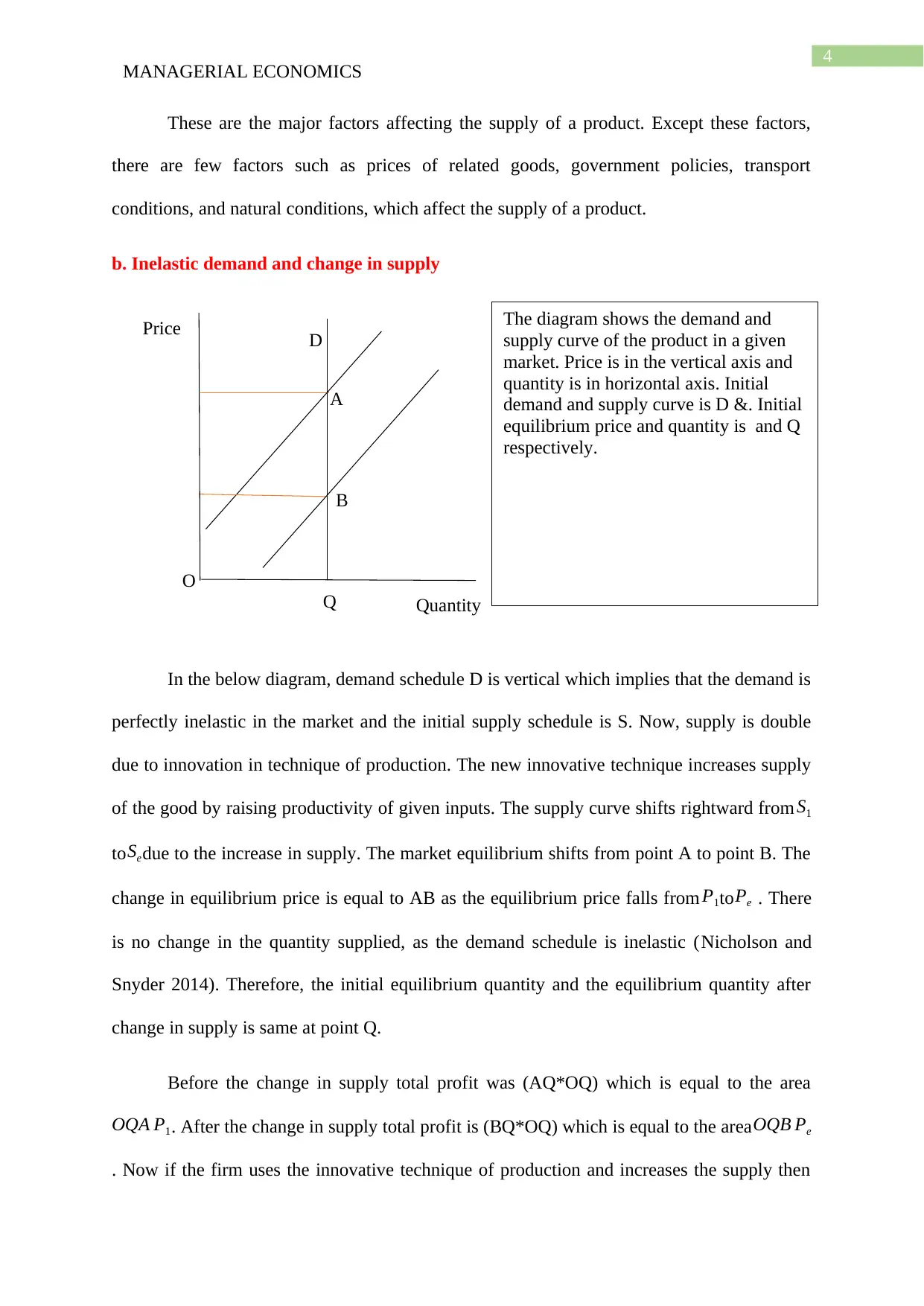
MANAGERIAL ECONOMICS
Q
Price
Quantity
D
The diagram shows the demand and
supply curve of the product in a given
market. Price is in the vertical axis and
quantity is in horizontal axis. Initial
demand and supply curve is D &. Initial
equilibrium price and quantity is and Q
respectively.
A
B
O
These are the major factors affecting the supply of a product. Except these factors,
there are few factors such as prices of related goods, government policies, transport
conditions, and natural conditions, which affect the supply of a product.
b. Inelastic demand and change in supply
In the below diagram, demand schedule D is vertical which implies that the demand is
perfectly inelastic in the market and the initial supply schedule is S. Now, supply is double
due to innovation in technique of production. The new innovative technique increases supply
of the good by raising productivity of given inputs. The supply curve shifts rightward from S1
to Sedue to the increase in supply. The market equilibrium shifts from point A to point B. The
change in equilibrium price is equal to AB as the equilibrium price falls from P1toPe . There
is no change in the quantity supplied, as the demand schedule is inelastic (Nicholson and
Snyder 2014). Therefore, the initial equilibrium quantity and the equilibrium quantity after
change in supply is same at point Q.
Before the change in supply total profit was (AQ*OQ) which is equal to the area
OQA P1. After the change in supply total profit is (BQ*OQ) which is equal to the area OQB Pe
. Now if the firm uses the innovative technique of production and increases the supply then
5
MANAGERIAL ECONOMICS
the firm has to face a decline in profit, which is equal to the area (
OQA P1−OQB Pe=P1 Pe BA). So, increment in the supply cannot be recommended to the
firm (Blad and Keiding 2014). However, the firm can use the innovative technique of
production to reduce the cost of production not to increase the supply.
Answer 2:
The three common used measure of elasticity of demand are price elasticity of
demand, income elasticity of demand and cross price elasticity of demand (Mahanty 2014).
Price elasticity of demand is defined by the percentage change in quantity demand
due to 1% change in price. It can be expressed mathematically as follows:
Depending on nature of the product and other determinant factors, elasticity ranges
from 0 to infinity.
Degrees of Price Elasticity:
The change in quantity depending on price is more or less or equals to zero. The
following points explain this categorical feature:
Perfectly Elastic Demand:
A small change in price leads to an infinite change in quantity demand is counted in this
degree of price elasticity. It is called perfectly elastic demand. In other words, if there is a
little rise in price, the demand will fall to zero (Thompson 2016). The perfectly elastic
demand curve will be horizontal straight line and ed =0.
Perfectly Inelastic Demand:
Perfectly inelastic demand implies a demand implies a demand situation where demand
remains completely ineffective for any change in price. Consumers’ here show no price
⊘ This is a preview!⊘
Do you want full access?
Subscribe today to unlock all pages.
Trusted by 1+ million students worldwide

6
MANAGERIAL ECONOMICS
sensitivity. The value of demand elasticity is zero. The corresponding demand curve is a
vertical straight line at the fixed quantity.
Unitary Elastic Demand:
There will be a same proportionate change in quantity demand due to a given proportionate
change in price. This is called unitary elastic demand. Simply, proportionate change in price
is equal to the proportionate change in demand. The unitary elastic demand curve will be
rectangular hyperbola and ed =1.
Relatively Elastic Demand:
There will be a relatively big change in quantity demand due to a small change in price.
This is called relatively elastic demand (Stoneman, Bartolon and Baussola 2018). In this case,
change in price has a greater impact on quantity demand. The relatively elastic demand curve
is relatively flatter and ed >1.
Relatively Inelastic Demand:
There will be a relatively small change in quantity demand due to a given change in
price. This is called relatively inelastic demand. In this case, change in price has a smaller
impact on quantity demand. The relatively inelastic demand curve is relatively stepper and
ed <1.
Point Elasticity Method:
Point elasticity method is nothing but the elasticity defined at a point not in average or
in percentage.
The formula for elasticity of demand using the mid-point method are given as follows
Paraphrase This Document
Need a fresh take? Get an instant paraphrase of this document with our AI Paraphraser
7
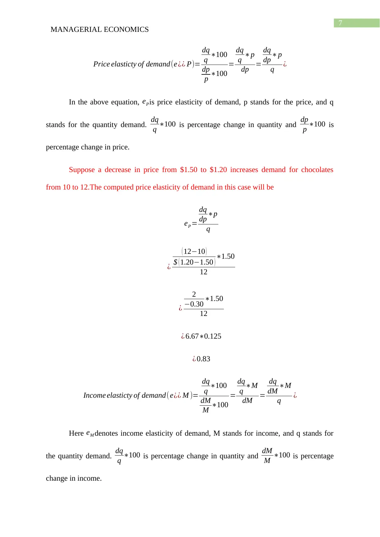
MANAGERIAL ECONOMICS
Price elasticty of demand(e ¿¿ P)=
dq
q ∗100
dp
p ∗100
=
dq
q ∗p
dp =
dq
dp ∗p
q ¿
In the above equation, ePis price elasticity of demand, p stands for the price, and q
stands for the quantity demand. dq
q ∗100 is percentage change in quantity and dp
p ∗100 is
percentage change in price.
Suppose a decrease in price from $1.50 to $1.20 increases demand for chocolates
from 10 to 12.The computed price elasticity of demand in this case will be
eP =
dq
dp ∗p
q
¿
( 12−10 )
$ ( 1.20−1.50 ) ∗1.50
12
¿
2
−0.30 ∗1.50
12
¿ 6.67∗0.125
¿ 0.83
Income elasticty of demand( e¿¿ M )=
dq
q ∗100
dM
M ∗100
=
dq
q ∗M
dM =
dq
dM ∗M
q ¿
Here eM denotes income elasticity of demand, M stands for income, and q stands for
the quantity demand. dq
q ∗100 is percentage change in quantity and dM
M ∗100 is percentage
change in income.
8
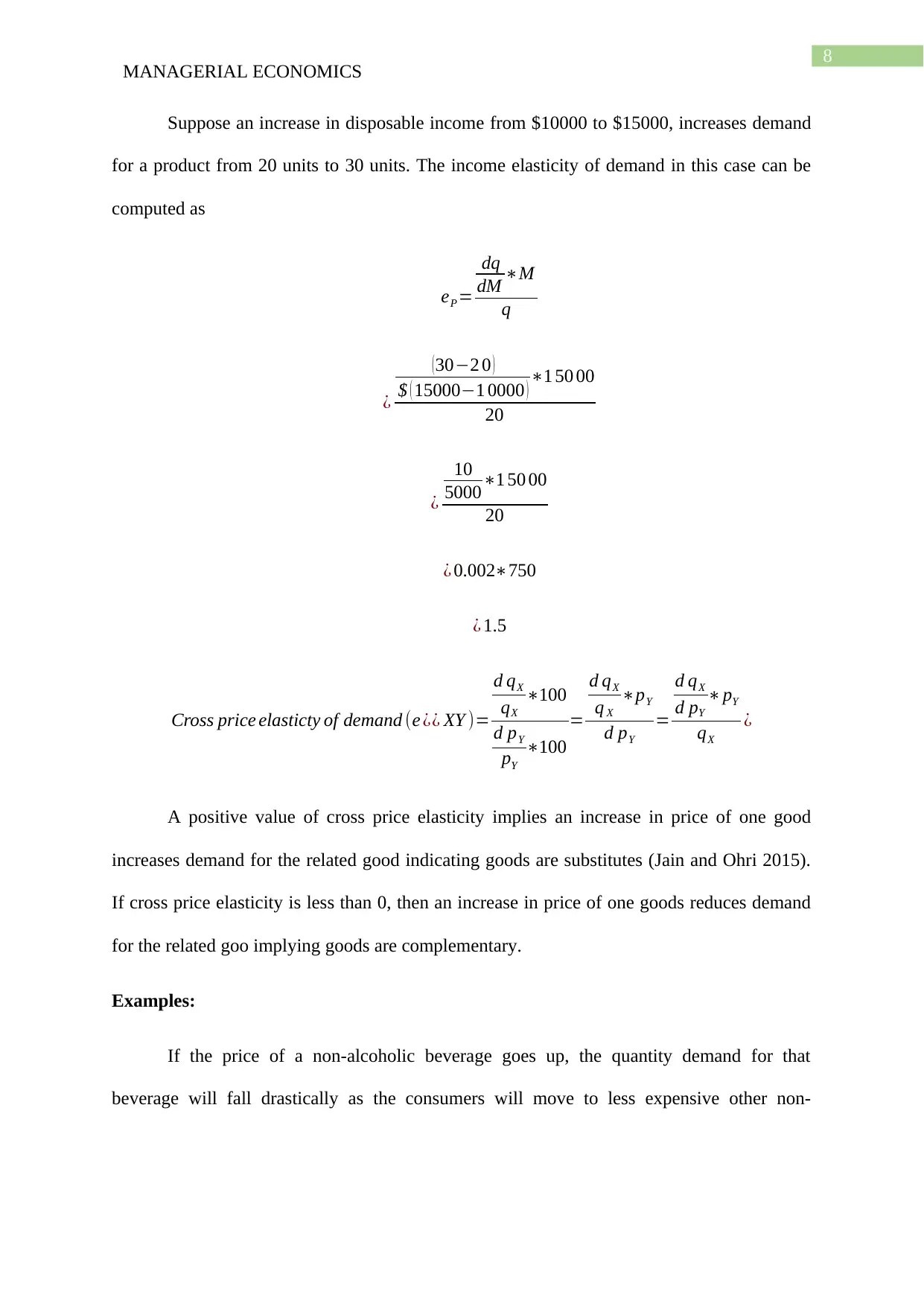
MANAGERIAL ECONOMICS
Suppose an increase in disposable income from $10000 to $15000, increases demand
for a product from 20 units to 30 units. The income elasticity of demand in this case can be
computed as
eP =
dq
dM ∗M
q
¿
(30−2 0 )
$ ( 15000−1 0000 ) ∗1 50 00
20
¿
10
5000∗1 50 00
20
¿ 0.002∗750
¿ 1.5
Cross price elasticty of demand (e ¿¿ XY )=
d qX
qX
∗100
d pY
pY
∗100
=
d qX
q X
∗pY
d pY
=
d qX
d pY
∗pY
qX
¿
A positive value of cross price elasticity implies an increase in price of one good
increases demand for the related good indicating goods are substitutes (Jain and Ohri 2015).
If cross price elasticity is less than 0, then an increase in price of one goods reduces demand
for the related goo implying goods are complementary.
Examples:
If the price of a non-alcoholic beverage goes up, the quantity demand for that
beverage will fall drastically as the consumers will move to less expensive other non-
⊘ This is a preview!⊘
Do you want full access?
Subscribe today to unlock all pages.
Trusted by 1+ million students worldwide
9
MANAGERIAL ECONOMICS
Price
Quantity
S
alcoholic beverages. Here, change in price reduces the demand in a large scale. Therefore, the
product is elastic.
If the price of gasoline goes up, the quantity demand will fall but in a small range.
The consumers have comparatively less substitutes for gasoline and they will buy gasoline at
comparatively high price (Mankiw 2014). Here, change in price reduces the demand in small
scale. Therefore, the product is inelastic.
Answer 4:
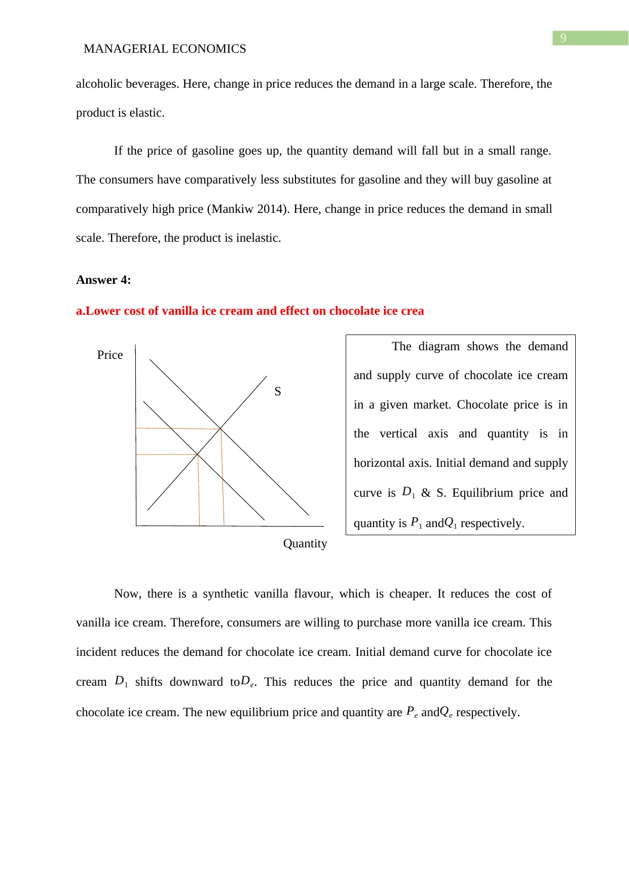
a.Lower cost of vanilla ice cream and effect on chocolate ice crea
Now, there is a synthetic vanilla flavour, which is cheaper. It reduces the cost of
vanilla ice cream. Therefore, consumers are willing to purchase more vanilla ice cream. This
incident reduces the demand for chocolate ice cream. Initial demand curve for chocolate ice
cream D1 shifts downward toDe. This reduces the price and quantity demand for the
chocolate ice cream. The new equilibrium price and quantity are Pe andQe respectively.
The diagram shows the demand
and supply curve of chocolate ice cream
in a given market. Chocolate price is in
the vertical axis and quantity is in
horizontal axis. Initial demand and supply
curve is D1 & S. Equilibrium price and
quantity is P1 and Q1 respectively.
MANAGERIAL ECONOMICS
Price
Quantity
S
alcoholic beverages. Here, change in price reduces the demand in a large scale. Therefore, the
product is elastic.
If the price of gasoline goes up, the quantity demand will fall but in a small range.
The consumers have comparatively less substitutes for gasoline and they will buy gasoline at
comparatively high price (Mankiw 2014). Here, change in price reduces the demand in small
scale. Therefore, the product is inelastic.
Answer 4:
a.Lower cost of vanilla ice cream and effect on chocolate ice crea
Now, there is a synthetic vanilla flavour, which is cheaper. It reduces the cost of
vanilla ice cream. Therefore, consumers are willing to purchase more vanilla ice cream. This
incident reduces the demand for chocolate ice cream. Initial demand curve for chocolate ice
cream D1 shifts downward toDe. This reduces the price and quantity demand for the
chocolate ice cream. The new equilibrium price and quantity are Pe andQe respectively.
The diagram shows the demand
and supply curve of chocolate ice cream
in a given market. Chocolate price is in
the vertical axis and quantity is in
horizontal axis. Initial demand and supply
curve is D1 & S. Equilibrium price and
quantity is P1 and Q1 respectively.
Paraphrase This Document
Need a fresh take? Get an instant paraphrase of this document with our AI Paraphraser
10
MANAGERIAL ECONOMICS
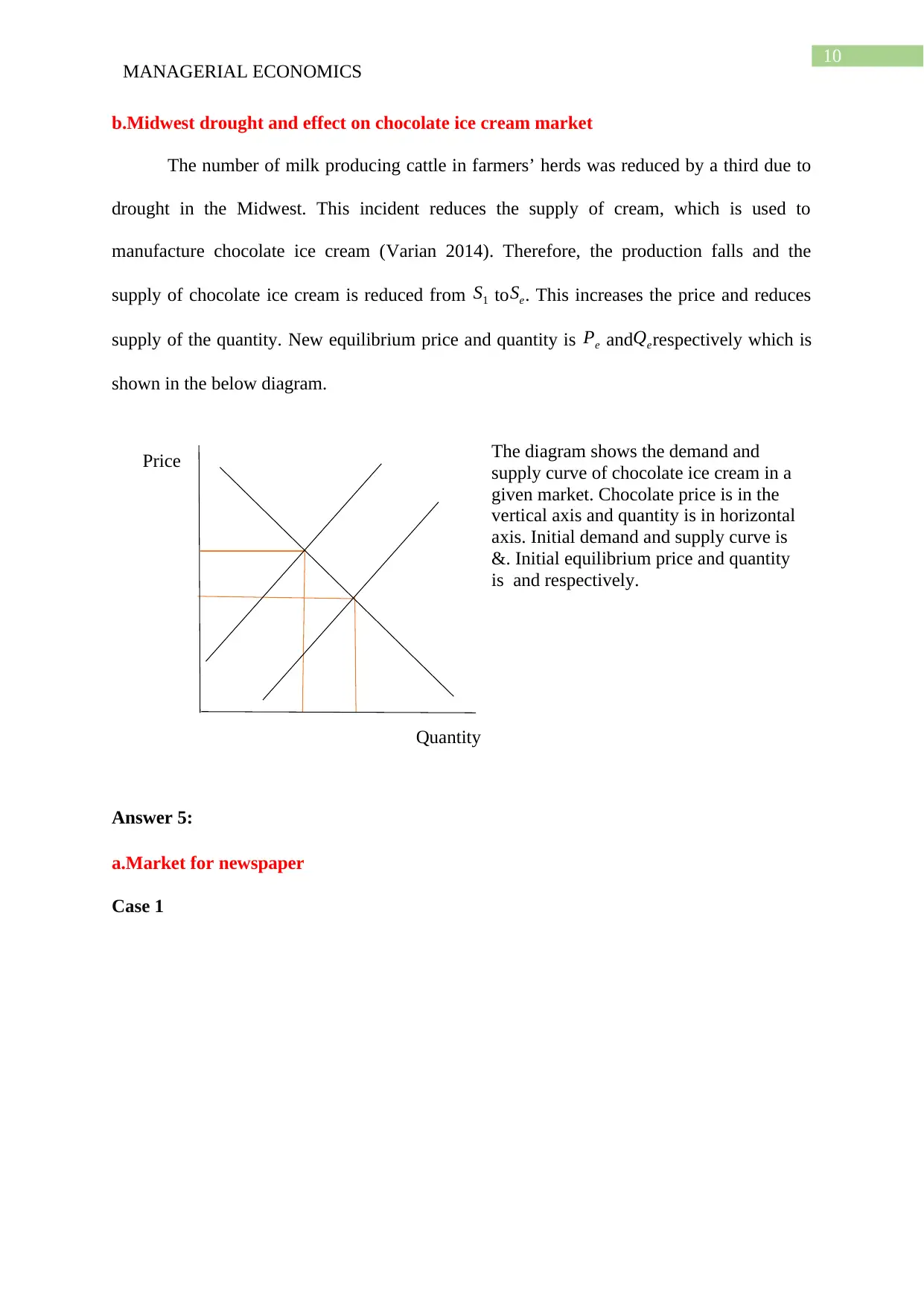
Price
Quantity
The diagram shows the demand and
supply curve of chocolate ice cream in a
given market. Chocolate price is in the
vertical axis and quantity is in horizontal
axis. Initial demand and supply curve is
&. Initial equilibrium price and quantity
is and respectively.
b.Midwest drought and effect on chocolate ice cream market
The number of milk producing cattle in farmers’ herds was reduced by a third due to
drought in the Midwest. This incident reduces the supply of cream, which is used to
manufacture chocolate ice cream (Varian 2014). Therefore, the production falls and the
supply of chocolate ice cream is reduced from S1 to Se. This increases the price and reduces
supply of the quantity. New equilibrium price and quantity is Pe andQerespectively which is
shown in the below diagram.
Answer 5:
a.Market for newspaper
Case 1
MANAGERIAL ECONOMICS
Price
Quantity
The diagram shows the demand and
supply curve of chocolate ice cream in a
given market. Chocolate price is in the
vertical axis and quantity is in horizontal
axis. Initial demand and supply curve is
&. Initial equilibrium price and quantity
is and respectively.
b.Midwest drought and effect on chocolate ice cream market
The number of milk producing cattle in farmers’ herds was reduced by a third due to
drought in the Midwest. This incident reduces the supply of cream, which is used to
manufacture chocolate ice cream (Varian 2014). Therefore, the production falls and the
supply of chocolate ice cream is reduced from S1 to Se. This increases the price and reduces
supply of the quantity. New equilibrium price and quantity is Pe andQerespectively which is
shown in the below diagram.
Answer 5:
a.Market for newspaper
Case 1
11
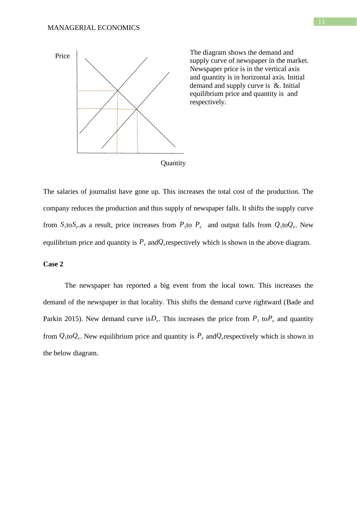
MANAGERIAL ECONOMICS
Price
Quantity
The diagram shows the demand and
supply curve of newspaper in the market.
Newspaper price is in the vertical axis
and quantity is in horizontal axis. Initial
demand and supply curve is &. Initial
equilibrium price and quantity is and
respectively.
The salaries of journalist have gone up. This increases the total cost of the production. The
company reduces the production and thus supply of newspaper falls. It shifts the supply curve
from S1toSe.as a result, price increases from P1to Pe and output falls from Q1toQe. New
equilibrium price and quantity is Pe andQerespectively which is shown in the above diagram.
Case 2
The newspaper has reported a big event from the local town. This increases the
demand of the newspaper in that locality. This shifts the demand curve rightward (Bade and
Parkin 2015). New demand curve isDe. This increases the price from P1 toPe and quantity
from Q1toQe. New equilibrium price and quantity is Pe and Qerespectively which is shown in
the below diagram.
⊘ This is a preview!⊘
Do you want full access?
Subscribe today to unlock all pages.
Trusted by 1+ million students worldwide
1 out of 23
Related Documents


Your All-in-One AI-Powered Toolkit for Academic Success.
+13062052269
info@desklib.com
Available 24*7 on WhatsApp / Email
![[object Object]](/_next/static/media/star-bottom.7253800d.svg)
Unlock your academic potential
Copyright © 2020–2026 A2Z Services. All Rights Reserved. Developed and managed by ZUCOL.