Applying Cox-PH Model for Survival Analysis in R Statistics

This assignment provides a detailed solution to a survival analysis problem using R statistics, focusing on the Cox-PH model. The solution includes calculating the expected risk (cumulative incidence) of events based on different conditions using models derived from the provided R code. It further involves calculating the difference between predicted values from two models and fitting a linear regression model using this difference as the outcome. Finally, the assignment tests the squared semi-partial correlations and partial correlations for each variable in the linear regression model, selecting variables that statistically account for more than 1% of the observed variations. The code and results offer a comprehensive approach to analyzing survival data and understanding the impact of various covariates.

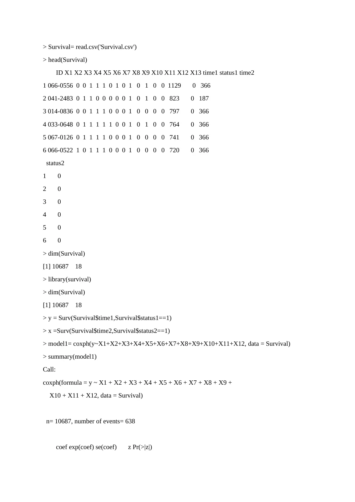
> Survival= read.csv('Survival.csv')
> head(Survival)
ID X1 X2 X3 X4 X5 X6 X7 X8 X9 X10 X11 X12 X13 time1 status1 time2
1 066-0556 0 0 1 1 1 0 1 0 1 0 1 0 0 1129 0 366
2 041-2483 0 1 1 0 0 0 0 0 1 0 1 0 0 823 0 187
3 014-0836 0 0 1 1 1 0 0 0 1 0 0 0 0 797 0 366
4 033-0648 0 1 1 1 1 1 0 0 1 0 1 0 0 764 0 366
5 067-0126 0 1 1 1 1 0 0 0 1 0 0 0 0 741 0 366
6 066-0522 1 0 1 1 1 0 0 0 1 0 0 0 0 720 0 366
status2
1 0
2 0
3 0
4 0
5 0
6 0
> dim(Survival)
[1] 10687 18
> library(survival)
> dim(Survival)
[1] 10687 18
> y = Surv(Survival$time1,Survival$status1==1)
> x =Surv(Survival$time2,Survival$status2==1)
> model1= coxph(y~X1+X2+X3+X4+X5+X6+X7+X8+X9+X10+X11+X12, data = Survival)
> summary(model1)
Call:
coxph(formula = y ~ X1 + X2 + X3 + X4 + X5 + X6 + X7 + X8 + X9 +
X10 + X11 + X12, data = Survival)
n= 10687, number of events= 638
coef exp(coef) se(coef) z Pr(>|z|)

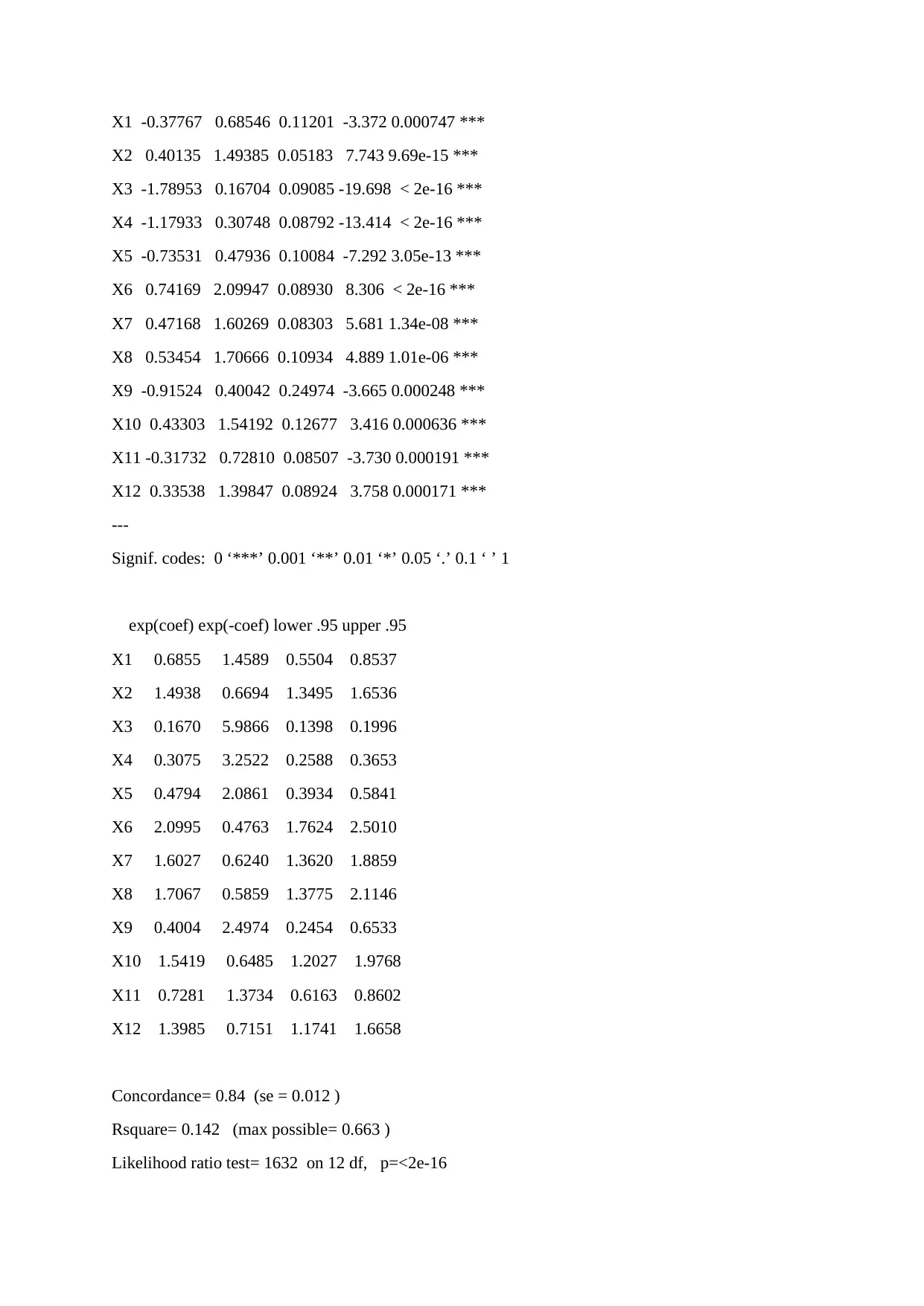
X1 -0.37767 0.68546 0.11201 -3.372 0.000747 ***
X2 0.40135 1.49385 0.05183 7.743 9.69e-15 ***
X3 -1.78953 0.16704 0.09085 -19.698 < 2e-16 ***
X4 -1.17933 0.30748 0.08792 -13.414 < 2e-16 ***
X5 -0.73531 0.47936 0.10084 -7.292 3.05e-13 ***
X6 0.74169 2.09947 0.08930 8.306 < 2e-16 ***
X7 0.47168 1.60269 0.08303 5.681 1.34e-08 ***
X8 0.53454 1.70666 0.10934 4.889 1.01e-06 ***
X9 -0.91524 0.40042 0.24974 -3.665 0.000248 ***
X10 0.43303 1.54192 0.12677 3.416 0.000636 ***
X11 -0.31732 0.72810 0.08507 -3.730 0.000191 ***
X12 0.33538 1.39847 0.08924 3.758 0.000171 ***
---
Signif. codes: 0 ‘***’ 0.001 ‘**’ 0.01 ‘*’ 0.05 ‘.’ 0.1 ‘ ’ 1
exp(coef) exp(-coef) lower .95 upper .95
X1 0.6855 1.4589 0.5504 0.8537
X2 1.4938 0.6694 1.3495 1.6536
X3 0.1670 5.9866 0.1398 0.1996
X4 0.3075 3.2522 0.2588 0.3653
X5 0.4794 2.0861 0.3934 0.5841
X6 2.0995 0.4763 1.7624 2.5010
X7 1.6027 0.6240 1.3620 1.8859
X8 1.7067 0.5859 1.3775 2.1146
X9 0.4004 2.4974 0.2454 0.6533
X10 1.5419 0.6485 1.2027 1.9768
X11 0.7281 1.3734 0.6163 0.8602
X12 1.3985 0.7151 1.1741 1.6658
Concordance= 0.84 (se = 0.012 )
Rsquare= 0.142 (max possible= 0.663 )
Likelihood ratio test= 1632 on 12 df, p=<2e-16

Wald test = 1911 on 12 df, p=<2e-16
Score (logrank) test = 3280 on 12 df, p=<2e-16
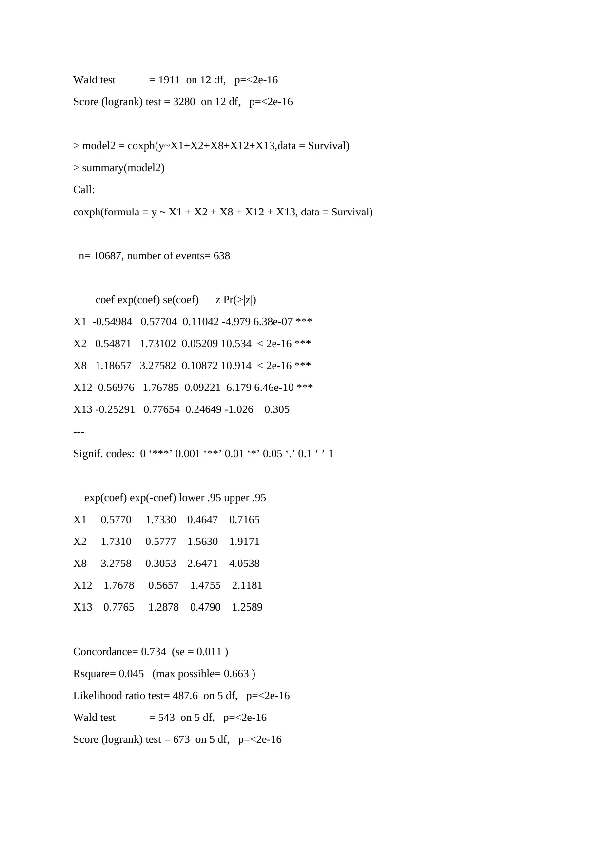
> model2 = coxph(y~X1+X2+X8+X12+X13,data = Survival)
> summary(model2)
Call:
coxph(formula = y ~ X1 + X2 + X8 + X12 + X13, data = Survival)
n= 10687, number of events= 638
coef exp(coef) se(coef) z Pr(>|z|)
X1 -0.54984 0.57704 0.11042 -4.979 6.38e-07 ***
X2 0.54871 1.73102 0.05209 10.534 < 2e-16 ***
X8 1.18657 3.27582 0.10872 10.914 < 2e-16 ***
X12 0.56976 1.76785 0.09221 6.179 6.46e-10 ***
X13 -0.25291 0.77654 0.24649 -1.026 0.305
---
Signif. codes: 0 ‘***’ 0.001 ‘**’ 0.01 ‘*’ 0.05 ‘.’ 0.1 ‘ ’ 1
exp(coef) exp(-coef) lower .95 upper .95
X1 0.5770 1.7330 0.4647 0.7165
X2 1.7310 0.5777 1.5630 1.9171
X8 3.2758 0.3053 2.6471 4.0538
X12 1.7678 0.5657 1.4755 2.1181
X13 0.7765 1.2878 0.4790 1.2589
Concordance= 0.734 (se = 0.011 )
Rsquare= 0.045 (max possible= 0.663 )
Likelihood ratio test= 487.6 on 5 df, p=<2e-16
Wald test = 543 on 5 df, p=<2e-16
Score (logrank) test = 673 on 5 df, p=<2e-16

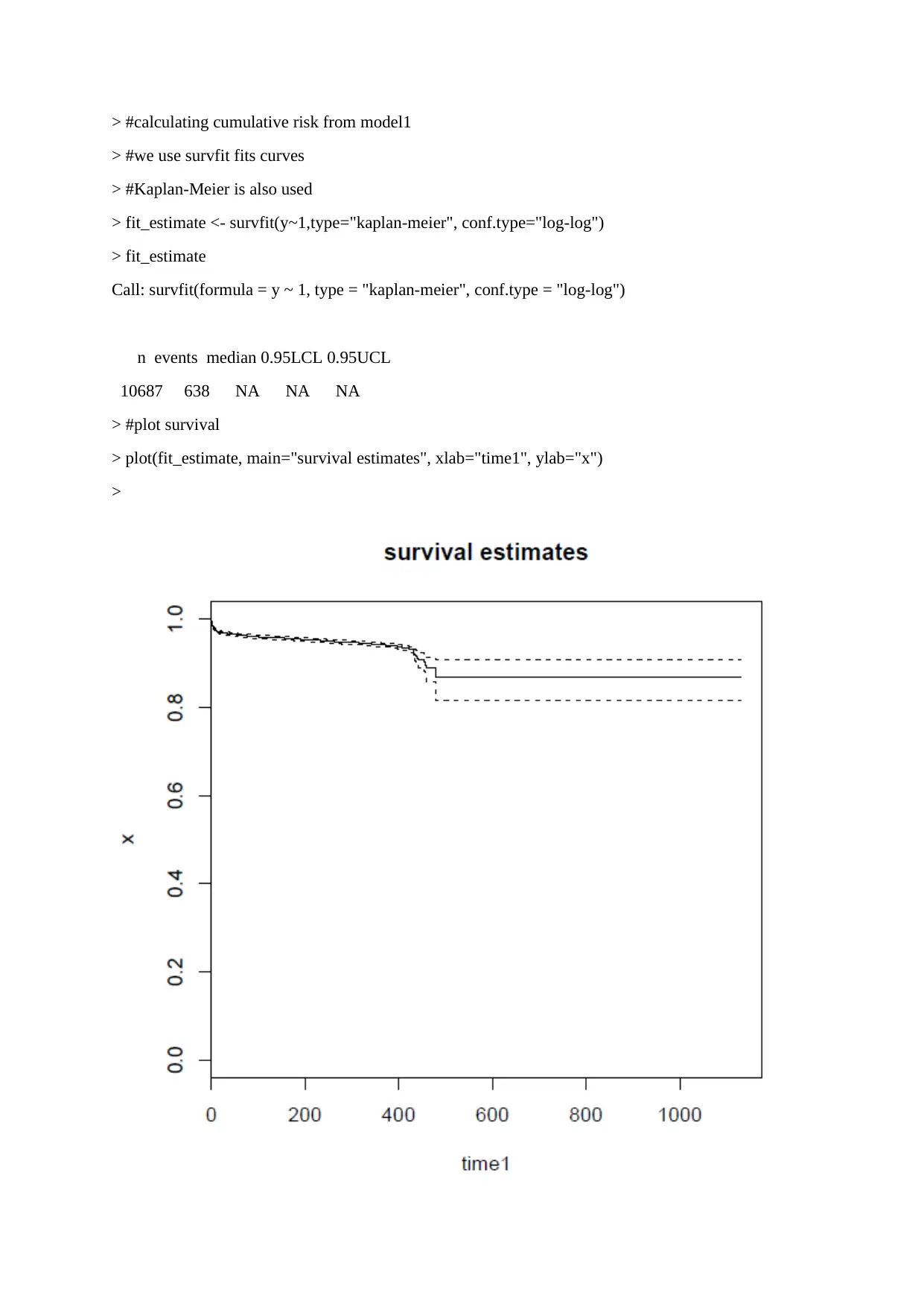
> #calculating cumulative risk from model1
> #we use survfit fits curves
> #Kaplan-Meier is also used
> fit_estimate <- survfit(y~1,type="kaplan-meier", conf.type="log-log")
> fit_estimate
Call: survfit(formula = y ~ 1, type = "kaplan-meier", conf.type = "log-log")
n events median 0.95LCL 0.95UCL
10687 638 NA NA NA
> #plot survival
> plot(fit_estimate, main="survival estimates", xlab="time1", ylab="x")
>

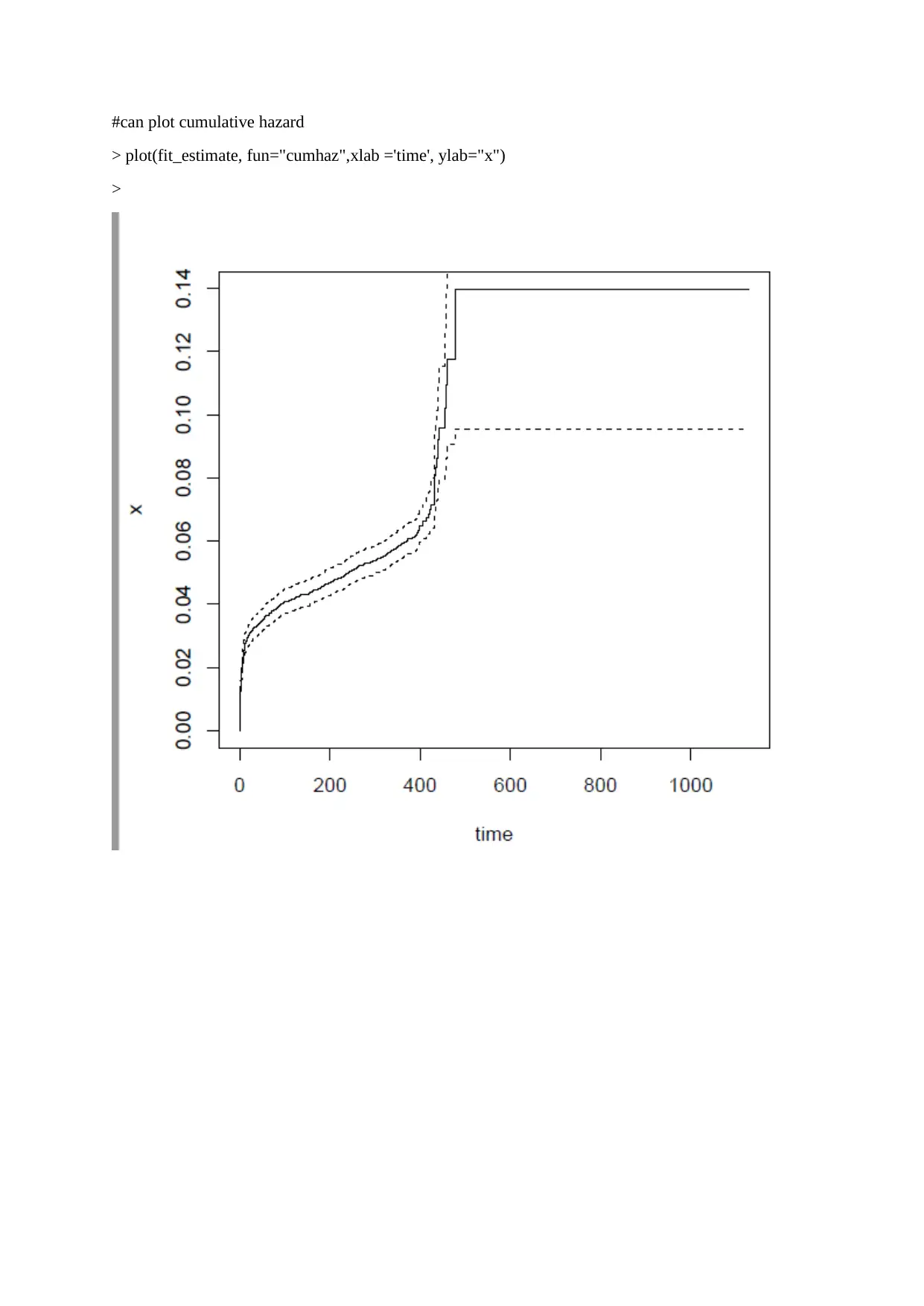
#can plot cumulative hazard
> plot(fit_estimate, fun="cumhaz",xlab ='time', ylab="x")
>