Systems Reliability Assignment Solutions - Professor Stupples, C125
VerifiedAdded on 2022/08/27
|19
|2479
|8
Homework Assignment
AI Summary
This document presents a comprehensive solution to a Systems Reliability assignment. It begins with fault tree analysis, deriving logical expressions for gate outputs, minimal cut sets, and calculating upper and lower bounds for the top event's probability using the inclusion-exclusion theorem. The assignment then delves into geothermal power unit reliability, calculating unavailability, mean time to failure, and sketching cumulative failure probability. Further, the solution explores the exponential distribution, hazard rate estimation, and confidence intervals for the mean time to failure. It includes graphical analysis of cumulative failure probability and discusses model suitability. The assignment also addresses the preference for constant failure rates in reliability calculations, convolution functions, and preventive maintenance strategies, drawing conclusions from an article on the subject and suggesting modifications to reliability analysis. Finally, it provides detailed calculations, interpretations, and reasoned arguments for each question, demonstrating a thorough understanding of systems reliability principles.

1
System Reliability
Name
Institution Affiliation
System Reliability
Name
Institution Affiliation
Paraphrase This Document
Need a fresh take? Get an instant paraphrase of this document with our AI Paraphraser
2
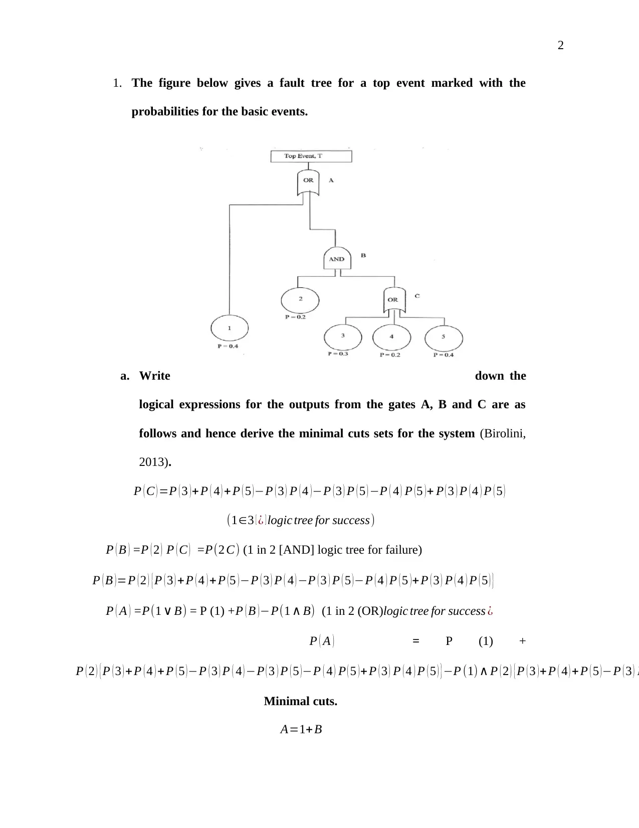
1. The figure below gives a fault tree for a top event marked with the
probabilities for the basic events.
a. Write down the
logical expressions for the outputs from the gates A, B and C are as
follows and hence derive the minimal cuts sets for the system (Birolini,
2013).
P ( C ) =P ( 3 )+ P ( 4 ) +P ( 5 )−P ( 3 ) P ( 4 )−P ( 3 ) P ( 5 ) −P ( 4 ) P (5 )+ P ( 3 ) P ( 4 ) P ( 5 )
(1∈3 [ ¿ ] logic tree for success)
P ( B ) =P ( 2 ) P ( C ) =P(2 C) (1 in 2 [AND] logic tree for failure)
P ( B )=P ( 2 ) {P ( 3 ) +P ( 4 ) + P (5 )−P ( 3 ) P ( 4 ) −P ( 3 ) P ( 5 )−P ( 4 ) P ( 5 )+ P ( 3 ) P ( 4 ) P ( 5 ) }
P ( A ) = P(1 ∨ B) = P (1) + P ( B ) −P(1 ∧ B) (1 in 2 (OR)logic tree for success ¿
P ( A ) = P (1) +
P ( 2 ) { P ( 3 ) + P ( 4 ) + P ( 5 ) −P ( 3 ) P ( 4 ) −P ( 3 ) P ( 5 ) −P ( 4 ) P ( 5 ) + P ( 3 ) P ( 4 ) P ( 5 ) } −P (1) ∧ P ( 2 ) { P ( 3 ) + P ( 4 ) + P ( 5 ) −P ( 3 ) P
Minimal cuts.
A=1+ B
3
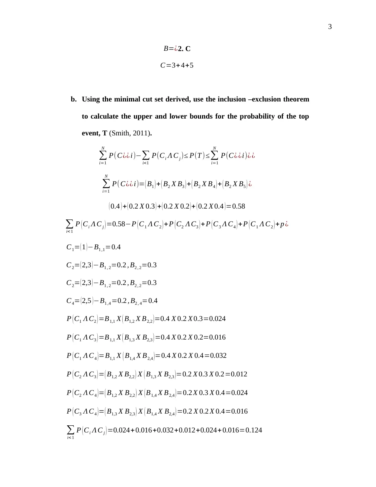
B=¿2. C
C=3+ 4+5
b. Using the minimal cut set derived, use the inclusion –exclusion theorem
to calculate the upper and lower bounds for the probability of the top
event, T (Smith, 2011).
∑
i=1
N
P(C¿¿ i)−∑
i<1
P(Ci Λ C j )≤ P(T )≤∑
i=1
N
P(C¿ ¿i)¿ ¿
∑
i=1
N
P( C¿¿ i)= ( B1 ) + ( B2 X B3 ) + ( B2 X B4 ) + ( B2 X B5 ) ¿
( 0.4 ) + ( 0.2 X 0.3 ) + ( 0.2 X 0.2 )+ ( 0.2 X 0.4 )=0.58
∑
i< 1
P ( Ci Λ C j ) =0.58−P ( C1 Λ C2 ) +P (C2 Λ C3 ) + P ( C3 Λ C4 ) +P ( C1 Λ C2 ) +p ¿
C1= ( 1 ) −B1 ,1=0.4
C2= ( 2,3 ) −B1 , 2=0.2 , B2 , 2=0.3
C2= ( 2,3 ) −B1 , 2=0.2 , B2 , 2=0.3
C4= ( 2,5 ) −B1 ,4 =0.2 , B2 , 4=0.4
P ( C1 Λ C2 ) =B1,1 X ( B1,2 X B2,2 ) =0.4 X 0.2 X 0.3=0.024
P ( C1 Λ C3 ) =B1,1 X ( B1,3 X B2,3 ) =0.4 X 0.2 X 0.2=0.016
P ( C1 Λ C4 )=B1,1 X ( B1,4 X B2,4 )=0.4 X 0.2 X 0.4=0.032
P ( C2 Λ C3 ) = ( B1,2 X B2,2 ) X ( B1,3 X B2,3 )=0.2 X 0.3 X 0.2=0.012
P ( C2 Λ C4 )= ( B1,2 X B2,2 ) X ( B1,4 X B2,4 ) =0.2 X 0.3 X 0.4=0.024
P ( C3 Λ C4 )= ( B1,3 X B2,3 ) X ( B1,4 X B2,4 ) =0.2 X 0.2 X 0.4=0.016
∑
i< 1
P ( Ci Λ C j ) =0.024+ 0.016+0.032+0.012+0.024+ 0.016=0.124
⊘ This is a preview!⊘
Do you want full access?
Subscribe today to unlock all pages.

Trusted by 1+ million students worldwide
4
∑
i=1
N
P(C¿¿ i)−∑
i<1
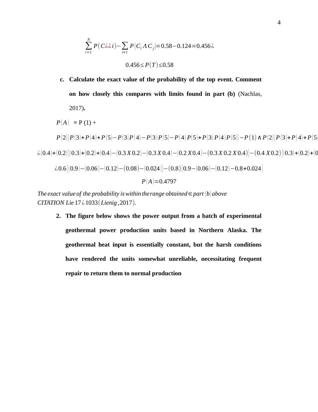
P ( Ci Λ C j )=0.58−0.124=0.456 ¿
0.456 ≤ P(T ) ≤0.58
c. Calculate the exact value of the probability of the top event. Comment
on how closely this compares with limits found in part (b) (Nachlas,
2017).
P ( A ) = P (1) +
P ( 2 ) {P ( 3 ) + P ( 4 ) + P ( 5 )−P ( 3 ) P ( 4 ) −P ( 3 ) P ( 5 )−P ( 4 ) P ( 5 )+ P ( 3 ) P ( 4 ) P ( 5 ) }−P (1) ∧ P ( 2 ) {P ( 3 )+P ( 4 ) + P ( 5 )
¿ ( 0.4 )+ ( 0.2 ) { ( 0.3 ) + ( 0.2 ) + ( 0.4 )− ( 0.3 X 0.2 ) − ( 0.3 X 0.4 ) − ( 0.2 X 0.4 )−(0.3 X 0.2 X 0.4) }−(0.4 X 0.2) { ( 0.3 ) + ( 0.2 ) + ( 0
¿ 0.6 { ( 0.9 )− ( 0.06 )− ( 0.12 )−(0.08)− ( 0.024 ) }−(0.8) {0.9− ( 0.06 )− ( 0.12 ) −0.8+0.024 }
P ( A )=0.4797
The exact value of the probability is within therange obtained ∈ part ( b ) above
CITATION Lie 17 ¿ 1033(Lienig ,2017) .
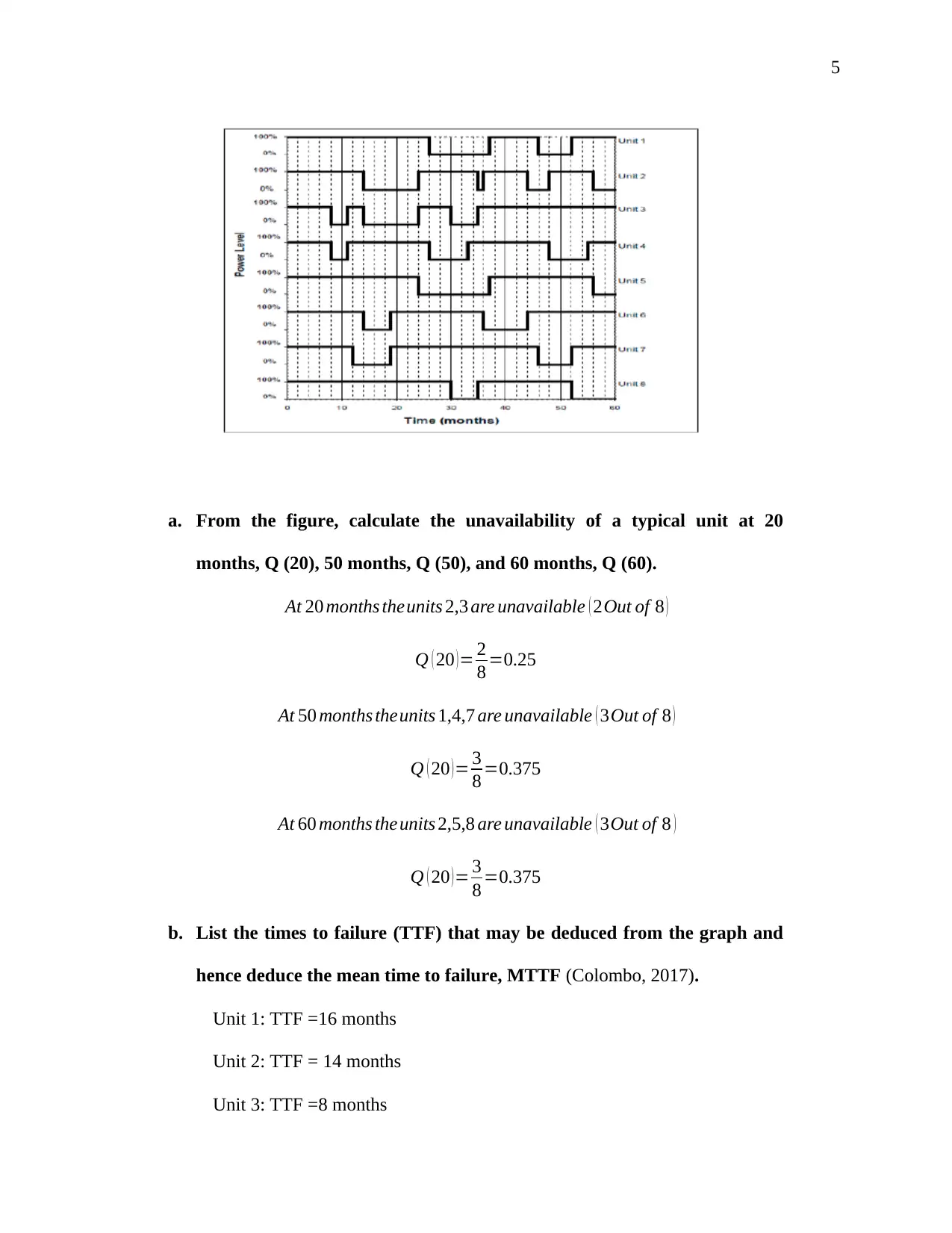
2. The figure below shows the power output from a batch of experimental
geothermal power production units based in Northern Alaska. The
geothermal heat input is essentially constant, but the harsh conditions
have rendered the units somewhat unreliable, necessitating frequent
repair to return them to normal production
Paraphrase This Document
Need a fresh take? Get an instant paraphrase of this document with our AI Paraphraser
5
a. From the figure, calculate the unavailability of a typical unit at 20
months, Q (20), 50 months, Q (50), and 60 months, Q (60).
At 20 months theunits 2,3 are unavailable ( 2Out of 8 )
Q ( 20 )= 2
8 =0.25
At 50 months theunits 1,4,7 are unavailable ( 3Out of 8 )
Q ( 20 )= 3
8 =0.375
At 60 months theunits 2,5,8 are unavailable ( 3Out of 8 )
Q ( 20 )= 3
8 =0.375
b. List the times to failure (TTF) that may be deduced from the graph and
hence deduce the mean time to failure, MTTF (Colombo, 2017).
Unit 1: TTF =16 months
Unit 2: TTF = 14 months
Unit 3: TTF =8 months
6
Unit 4: TTF = 8 months
Unit 5: TTF = 24months
Unit 6: TTF =14 months
Unit 7: TTF =12 months
Unit 8: TTF =27 months
MTTF= 135
8 =16.88
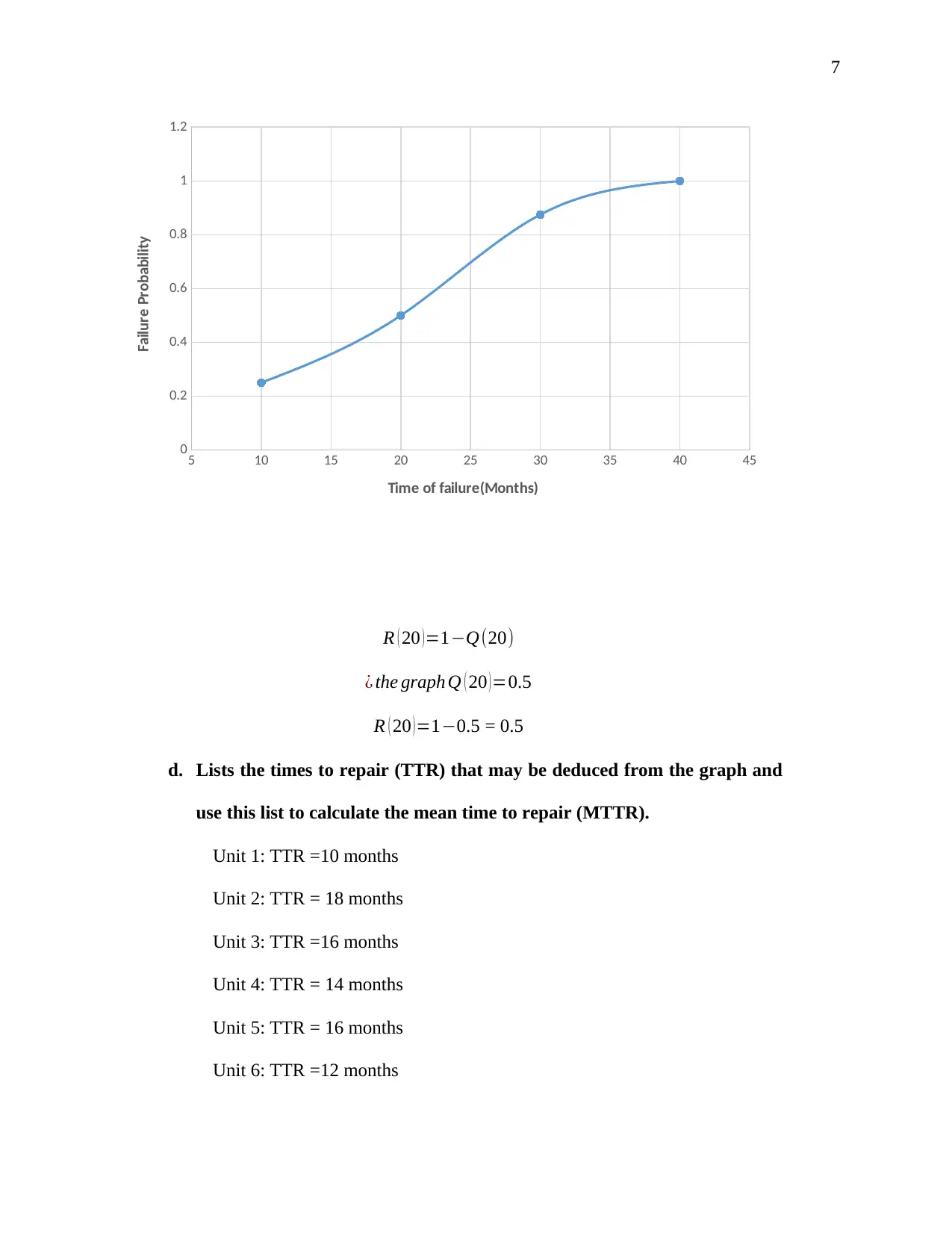
c. Using your data sketch of the cumulative failure probability/unreliability,
for a typical system as a function of running time over range 0 to 35
months. Estimate the reliability of a system that has been running for
20months, R (20) (JA1012, 2014).
Time of failure (months) Failure number Failure probability
10 2 0.25
20 4 0.5
30 7 0.875
40 8 1
⊘ This is a preview!⊘
Do you want full access?
Subscribe today to unlock all pages.

Trusted by 1+ million students worldwide
7
5 10 15 20 25 30 35 40 45
0
0.2
0.4
0.6
0.8
1
1.2
Time of failure(Months)
Failure Probability
R ( 20 ) =1−Q(20)
¿ the graph Q ( 20 )=0.5
R ( 20 )=1−0.5 = 0.5
d. Lists the times to repair (TTR) that may be deduced from the graph and
use this list to calculate the mean time to repair (MTTR).
Unit 1: TTR =10 months
Unit 2: TTR = 18 months
Unit 3: TTR =16 months
Unit 4: TTR = 14 months
Unit 5: TTR = 16 months
Unit 6: TTR =12 months
Paraphrase This Document
Need a fresh take? Get an instant paraphrase of this document with our AI Paraphraser
8
Unit 7: TTR =12 months
Unit 8: TTR =12 months
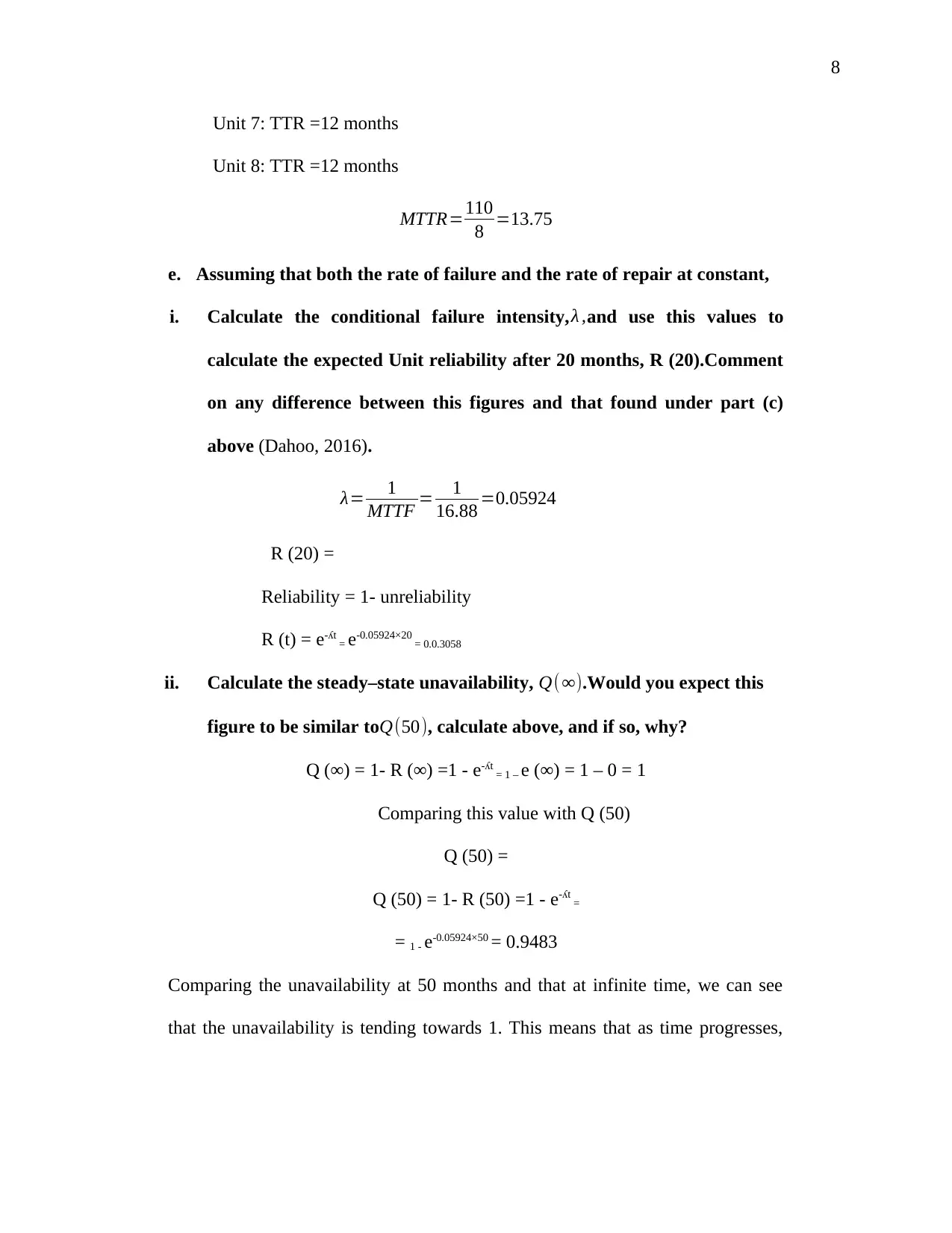
MTTR=110
8 =13.75
e. Assuming that both the rate of failure and the rate of repair at constant,
i. Calculate the conditional failure intensity, λ ,and use this values to
calculate the expected Unit reliability after 20 months, R (20).Comment
on any difference between this figures and that found under part (c)
above (Dahoo, 2016).
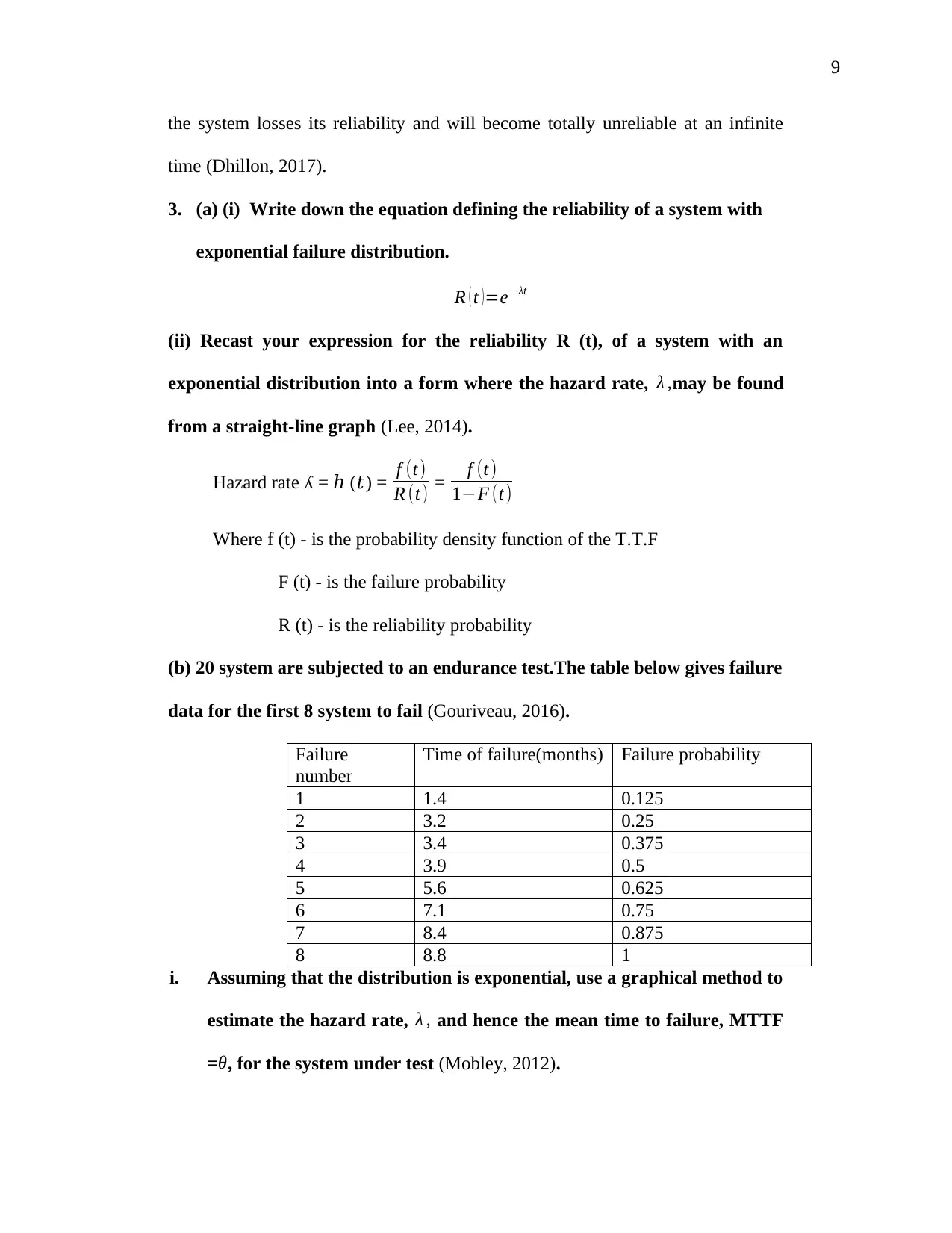
λ= 1
MTTF = 1
16.88 =0.05924
R (20) =
Reliability = 1- unreliability
R (t) = e-ʎt = e-0.05924×20 = 0.0.3058
ii. Calculate the steady–state unavailability, Q( ∞).Would you expect this
figure to be similar to Q(50), calculate above, and if so, why?
Q (∞) = 1- R (∞) =1 - e-ʎt = 1 – e (∞) = 1 – 0 = 1
Comparing this value with Q (50)
Q (50) =
Q (50) = 1- R (50) =1 - e-ʎt =
= 1 - e-0.05924×50 = 0.9483
Comparing the unavailability at 50 months and that at infinite time, we can see
that the unavailability is tending towards 1. This means that as time progresses,
9
the system losses its reliability and will become totally unreliable at an infinite
time (Dhillon, 2017).
3. (a) (i) Write down the equation defining the reliability of a system with
exponential failure distribution.
R ( t )=e− λt
(ii) Recast your expression for the reliability R (t), of a system with an
exponential distribution into a form where the hazard rate, λ ,may be found
from a straight-line graph (Lee, 2014).
Hazard rate ʎ = (ℎ 𝑡) = f (t)
R (t) = f (t )
1−F (t)
Where f (t) - is the probability density function of the T.T.F
F (t) - is the failure probability
R (t) - is the reliability probability
(b) 20 system are subjected to an endurance test.The table below gives failure
data for the first 8 system to fail (Gouriveau, 2016).
Failure
number
Time of failure(months) Failure probability
1 1.4 0.125
2 3.2 0.25
3 3.4 0.375
4 3.9 0.5
5 5.6 0.625
6 7.1 0.75
7 8.4 0.875
8 8.8 1
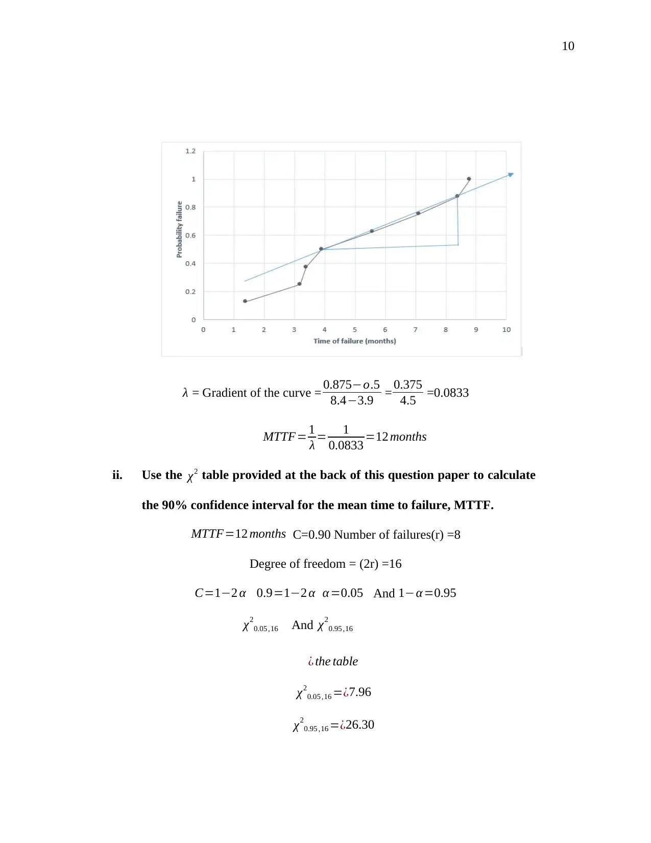
i. Assuming that the distribution is exponential, use a graphical method to
estimate the hazard rate, λ , and hence the mean time to failure, MTTF
=θ, for the system under test (Mobley, 2012).
⊘ This is a preview!⊘
Do you want full access?
Subscribe today to unlock all pages.

Trusted by 1+ million students worldwide
10
λ = Gradient of the curve = 0.875−o.5
8.4−3.9 = 0.375
4.5 =0.0833
MTTF= 1
λ = 1
0.0833 =12 months
ii. Use the χ2 table provided at the back of this question paper to calculate
the 90% confidence interval for the mean time to failure, MTTF.
MTTF=12 months C=0.90 Number of failures(r) =8
Degree of freedom = (2r) =16
C=1−2 α 0.9=1−2 α α =0.05 And 1−α =0.95
χ2
0.05 ,16 And χ2
0.95 ,16
¿ the table
χ2
0.05 ,16 =¿7.96
χ2
0.95 ,16 =¿26.30
Paraphrase This Document
Need a fresh take? Get an instant paraphrase of this document with our AI Paraphraser
11
θ0.95 =2 x 8 x 12
7.96 =24.12 months
θ0.95 =2 x 8 x 12
26.30 =7.3 months
7.3 ≤ MTTF ≤24.12
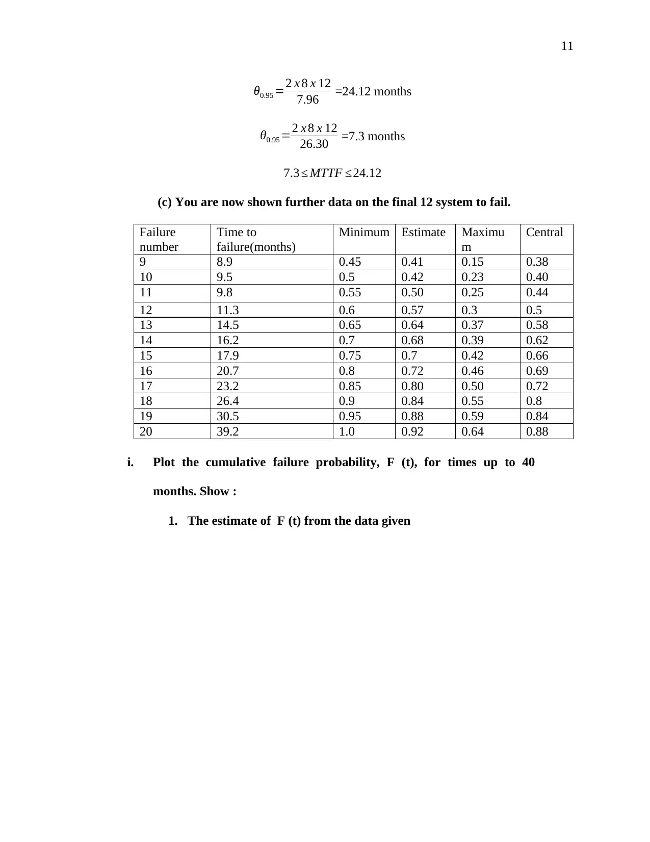
(c) You are now shown further data on the final 12 system to fail.
Failure
number
Time to
failure(months)
Minimum Estimate Maximu
m
Central
9 8.9 0.45 0.41 0.15 0.38
10 9.5 0.5 0.42 0.23 0.40
11 9.8 0.55 0.50 0.25 0.44
12 11.3 0.6 0.57 0.3 0.5
13 14.5 0.65 0.64 0.37 0.58
14 16.2 0.7 0.68 0.39 0.62
15 17.9 0.75 0.7 0.42 0.66
16 20.7 0.8 0.72 0.46 0.69
17 23.2 0.85 0.80 0.50 0.72
18 26.4 0.9 0.84 0.55 0.8
19 30.5 0.95 0.88 0.59 0.84
20 39.2 1.0 0.92 0.64 0.88
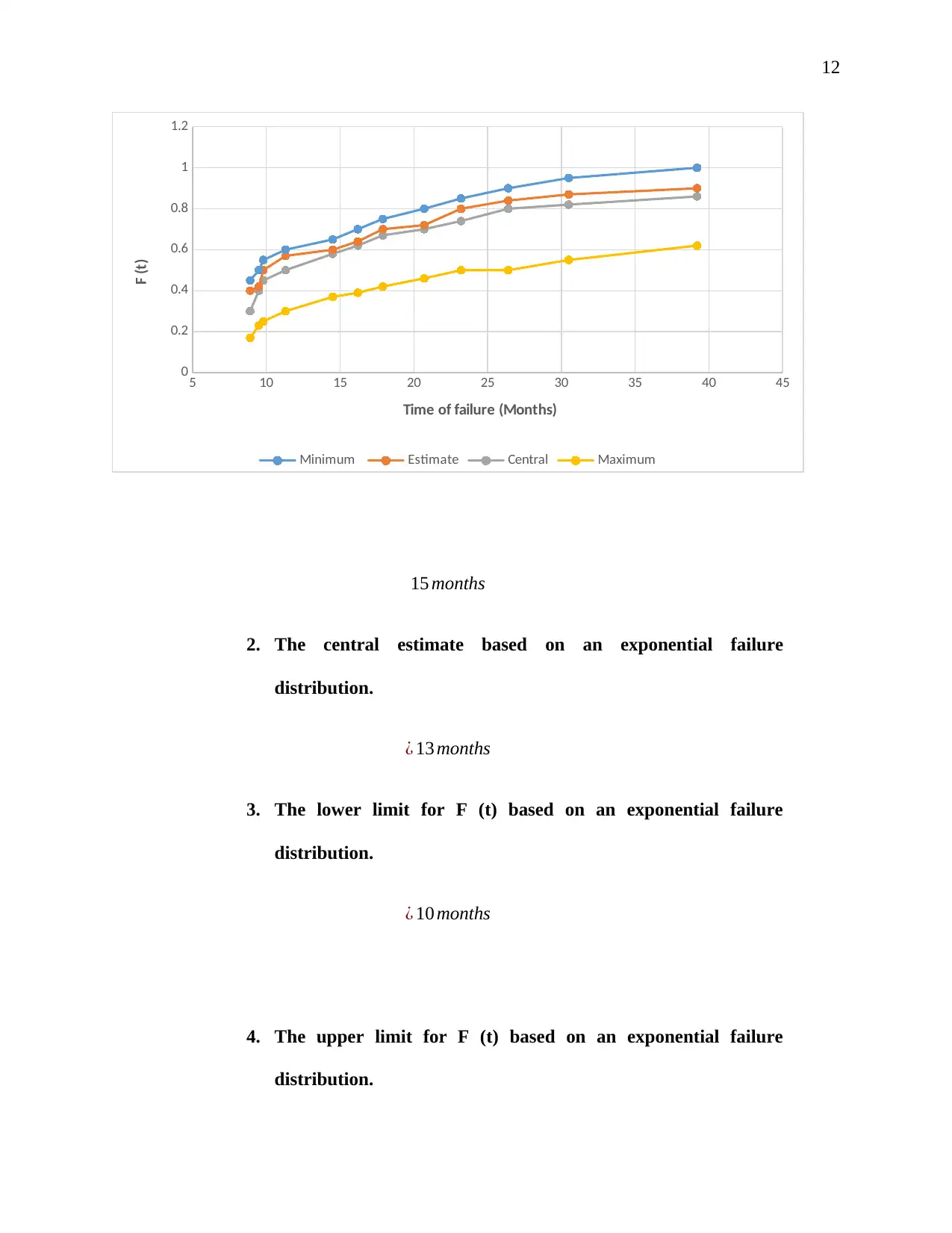
i. Plot the cumulative failure probability, F (t), for times up to 40
months. Show :
1. The estimate of F (t) from the data given
θ0.95 =2 x 8 x 12
7.96 =24.12 months
θ0.95 =2 x 8 x 12
26.30 =7.3 months
7.3 ≤ MTTF ≤24.12
(c) You are now shown further data on the final 12 system to fail.
Failure
number
Time to
failure(months)
Minimum Estimate Maximu
m
Central
9 8.9 0.45 0.41 0.15 0.38
10 9.5 0.5 0.42 0.23 0.40
11 9.8 0.55 0.50 0.25 0.44
12 11.3 0.6 0.57 0.3 0.5
13 14.5 0.65 0.64 0.37 0.58
14 16.2 0.7 0.68 0.39 0.62
15 17.9 0.75 0.7 0.42 0.66
16 20.7 0.8 0.72 0.46 0.69
17 23.2 0.85 0.80 0.50 0.72
18 26.4 0.9 0.84 0.55 0.8
19 30.5 0.95 0.88 0.59 0.84
20 39.2 1.0 0.92 0.64 0.88
i. Plot the cumulative failure probability, F (t), for times up to 40
months. Show :
1. The estimate of F (t) from the data given
12
5 10 15 20 25 30 35 40 45
0
0.2
0.4
0.6
0.8
1
1.2
Minimum Estimate Central Maximum
Time of failure (Months)
F (t)
15 months
2. The central estimate based on an exponential failure
distribution.
¿ 13 months
3. The lower limit for F (t) based on an exponential failure
distribution.
¿ 10 months
4. The upper limit for F (t) based on an exponential failure
distribution.
⊘ This is a preview!⊘
Do you want full access?
Subscribe today to unlock all pages.

Trusted by 1+ million students worldwide
1 out of 19
Your All-in-One AI-Powered Toolkit for Academic Success.
+13062052269
info@desklib.com
Available 24*7 on WhatsApp / Email
![[object Object]](/_next/static/media/star-bottom.7253800d.svg)
Unlock your academic potential
Copyright © 2020–2026 A2Z Services. All Rights Reserved. Developed and managed by ZUCOL.