Economics Assignment (Course ID: ECON101): Tax and Price Analysis

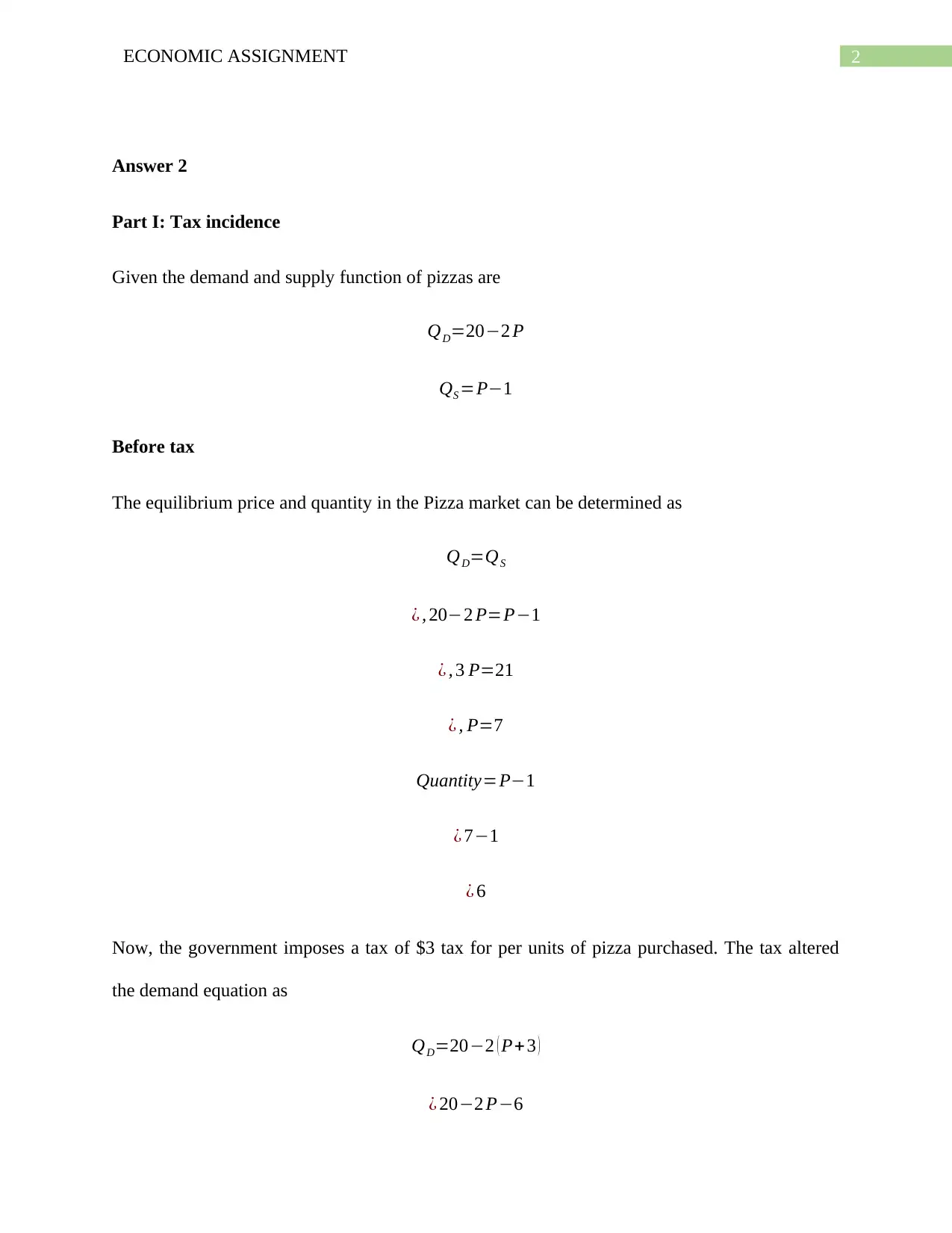
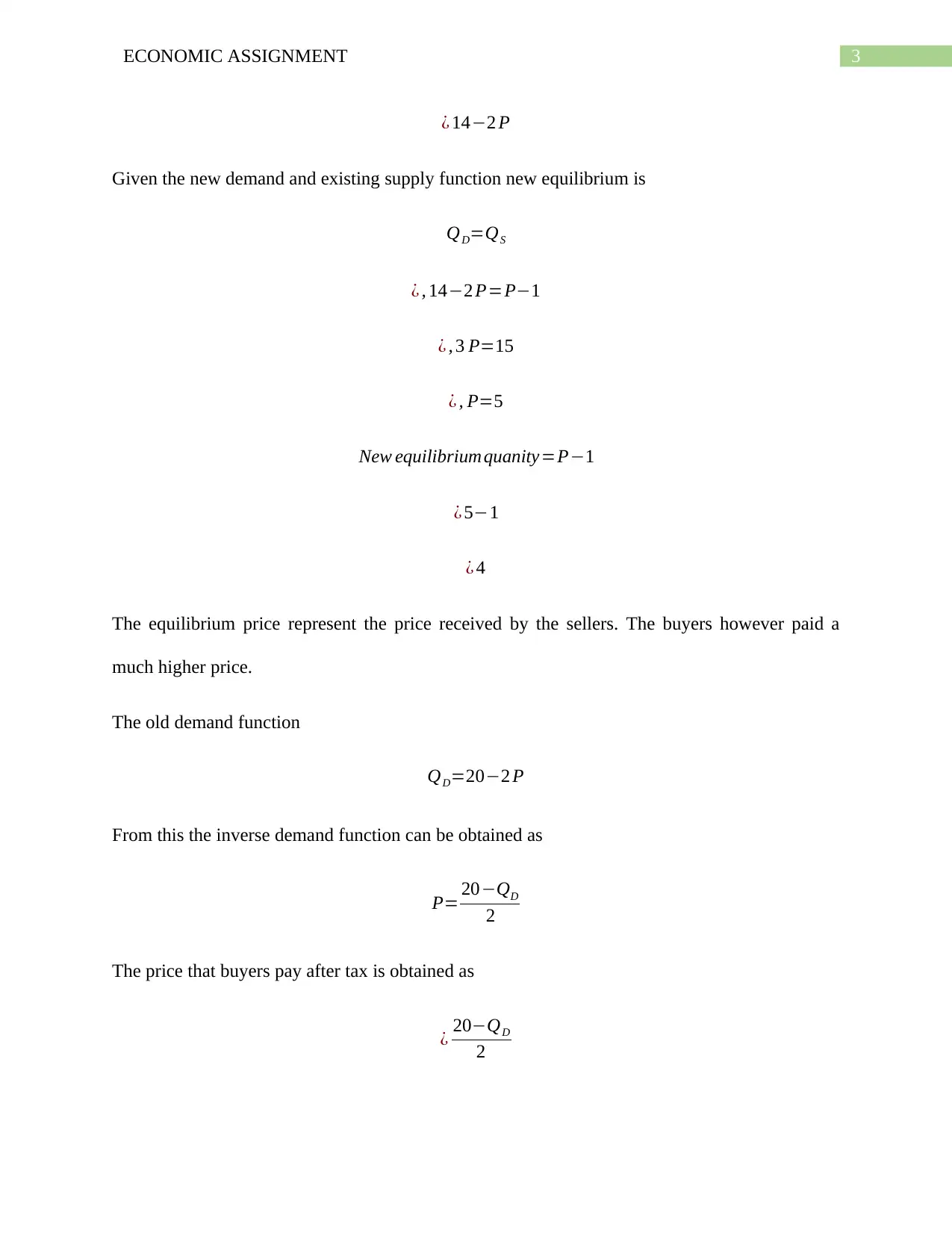
This economics assignment delves into two key areas: tax incidence and price regulation. Part I analyzes the impact of a per-unit tax on pizza, determining the new equilibrium price and quantity, the burden on buyers and sellers, and government revenue. The assignment utilizes supply and demand functions to illustrate these effects. Part II examines price regulation, specifically using the US Farm Bill as a case study. It assesses the impact of a price floor on the wheat market, including surplus generation, and analyzes changes in consumer surplus, producer surplus, and deadweight loss. The assignment also discusses the fairness implications of price intervention, highlighting how price supports can lead to market inefficiencies and uneven distribution of benefits, challenging the notion of equitable wealth transfer within the economic system. The assignment provides detailed calculations, graphical representations, and a discussion of the economic principles at play.

Running Head: ECONOMIC ASSIGNMENT
Economic Assignment
Name of the Student
Name of the University
Course ID

1ECONOMIC ASSIGNMENT
Table of Contents
Answer 2..........................................................................................................................................2
Part I: Tax incidence....................................................................................................................2
Part II: Price regulation................................................................................................................5
Answer a..................................................................................................................................5
Answer b..................................................................................................................................6
Answer c..................................................................................................................................6
Answer d..................................................................................................................................8
References......................................................................................................................................10

2ECONOMIC ASSIGNMENT
Answer 2
Part I: Tax incidence
Given the demand and supply function of pizzas are
QD=20−2 P
QS =P−1
Before tax
The equilibrium price and quantity in the Pizza market can be determined as
QD=QS
¿ , 20−2 P=P−1
¿ , 3 P=21
¿ , P=7
Quantity=P−1
¿ 7−1
¿ 6
Now, the government imposes a tax of $3 tax for per units of pizza purchased. The tax altered
the demand equation as
QD=20−2 ( P+ 3 )
¿ 20−2 P−6

3ECONOMIC ASSIGNMENT
¿ 14−2 P
Given the new demand and existing supply function new equilibrium is
QD=QS
¿ , 14−2 P=P−1
¿ , 3 P=15
¿ , P=5
New equilibrium quanity=P−1
¿ 5−1
¿ 4
The equilibrium price represent the price received by the sellers. The buyers however paid a
much higher price.
The old demand function
QD=20−2 P
From this the inverse demand function can be obtained as
P= 20−QD
2
The price that buyers pay after tax is obtained as
¿ 20−QD
2

4ECONOMIC ASSIGNMENT
¿ 20−4
2
¿ 16
2
¿ 8
Figure 1: Tax incidence in the Pizza market
The figure above can be used to understand the incidence of taxation. The downward sloping
curve DD shows demand curve for pizza and SS curve shows the corresponding supply curve.
As a result of $3 tax on per unit of pizza purchased, there is inward shift of the demand curve to
D’D’ (Taylor et al. 2014). Now, the price paid by buyers increases to $8 from initial equilibrium
price of $7. From the price paid by buyers, sellers receive only $5 and the rest goes to

5ECONOMIC ASSIGNMENT
government. The equilibrium number of pizzas in the market declined to 4 from initial
equilibrium of 6. Government receives a revenue of
($3*4) = $12. The burden to buyers is ($8 - $7) *4 = $4. The burden to seller is ($7 - $5) *4 = $8.
The buyers bear a less burden of taxation as compared to seller because of the relatively elastic
demand curve.
Part II: Price regulation
Answer a
Figure 2: Effect of US farm bill on Equilibrium
The equilibrium in the wheat market is at E. The price is at $250 with an equilibrium
quantity of 1000,000 tons of wheat. Under the Farm bill, price is set at $300, above the domestic
equilibrium price of $250. At $300, the supplied quantity of wheat is 1200,000 tons while
demanded quantity is 800,000 tons. In the market there exists a surplus of (1200,000 – 800,000)
= 400,000 tons of wheat.

6ECONOMIC ASSIGNMENT
Answer b
Figure 3: CS, PS and Deadweight loss
Under domestic equilibrium price of $250, the surplus to consumer is shown by the area
of the triangle ABE. The surplus to producer is the triangular area of BEC. As the price now
increases to $300, the consumer surplus now reduces to the triangle ADF. The new producer
surplus is equivalent to area of the trapezium DFHC. Part of the consumer surplus transferred to
producers. The dead weight loss is the area of the triangle EFH.
Answer c
Under domestic equilibrium the consumer and producer surplus can be computed as
Consumer Surplus(CS)=∆ ABE

7ECONOMIC ASSIGNMENT
¿ 1
2 × ( 400−250 ) ×1000000
¿ 75000000
Producer Surplus=∆ BEC
¿=1
2 × ( 250−100 ) × 1000000
¿ 75000000
Total surplus is the sum of consumer and producer surplus
Total surplus=CS+PS
¿ 75000000+75000000
¿ 150000000
With farm bill, the change in consumer surplus, producer surplus and resulted deadweight loss
can be calculated as
Consumer Surplus=∆ ADF
¿ 1
2 × ( 400−300 ) ×8000000
¿ 40000000
Change∈cosnumer surplus=75000000−40000000=35000000
Producer surplus=∆ DGC−∆ FGH
¿ 1
2 ×1200000 × ( 300−100 )− 1
2 × (300−200 ) × ( 1200000−800000 )

8ECONOMIC ASSIGNMENT
¿ 1
2 ×1200000 ×200−1
2 ×100 ×400000
¿ 120000000−20000000
¿ 100000000
Change∈ producer surplus=100000000−75000000=25000000
Total Surplus=40000000+100000000=140000000
Change∈total surplus=150000000−140000000=10000000
Deadweight loss=∆ E F H=2 × 1
2 × ( 300−250 ) × ( 1000000−800000 )
¿ 50 ×2000000
¿ 10000000
Answer d
The notion of fairness in economics implies that the wealth that is take out of the system
should be proportional to the contribution put into the system. Under any form of price
intervention, there is not absolute transfer of welfare from one party to another. Like in case of
US farm bill, price in the market artificially increases to $300. The buyers face a high price and
hence experiences a reduction in surplus. However, the reduced surplus does not completely
transfer to the farmers. The agricultural price support program results in a marketed surplus in
the economy. The surplus needs to be purchased by government (Frank 2015). This additional
burden of government budget is again fall on the buyers in form of a higher taxation. The surplus
to farmers though increases but at the cost of other groups in the society. The fruits of price

9ECONOMIC ASSIGNMENT
support program are not even fairly distributed among the farmers. Large farmers generally gain
at the expense of small and medium sized farmers. The result of US farm bill is thus not fair.

10ECONOMIC ASSIGNMENT
References
Frank, R.H., 2015. Principles of microeconomics, brief edition. Mcgraw-Hill.
Taylor, T., Greenlaw, S.A., Dodge, E.R., Gamez, C., Jauregui, A., Keenan, D., MacDonald, D.,
Moledina, A., Richardson, C., Shapiro, D. and Sonenshine, R., 2014. Principles of
microeconomics. OpenStax College, Rice University.

11ECONOMIC ASSIGNMENT