Scientific Report: Comparative Analysis of TEE in Groups A and B

This scientific report presents a comprehensive analysis of total energy expenditure (TEE) data, comparing two groups, A and B. The report includes an abstract, introduction, methods, discussion, and conclusion. Key methods employed are statistical analysis, t-tests for determining P-values, and correlation techniques to explore relationships between variables like TEE and body weight. The study aims to estimate TEE, predict resting metabolic rate (RMR), and assess physical activity levels (PAL). It also discusses the significance of RMR, metabolic equivalents (METs), and the use of the Physical Activities Compendium. The report provides detailed statistical analyses for both groups, including mean, variance, and correlation coefficients, offering insights into the relationships between different factors influencing energy expenditure. Finally, the report concludes by summarizing key findings and their implications.

Scientific Report Writing
1

ABSTRACT
The study summaries scientific analysis of given data of total energy expenditure which is
classified in two groups A and B. In study P values for Group A and Group B are determined
which help to assess the actual significance of data. Further the study comprises certain major
methods like statistical analysis, correlation etc. to better explore the relevance of study.
2

Contents
ABSTRACT.....................................................................................................................................2
Contents...........................................................................................................................................3
Introduction and Aim.......................................................................................................................4
Methods and Discussion..................................................................................................................4
Conclusion.....................................................................................................................................12
REFERENCES..............................................................................................................................13
Appendix........................................................................................................................................14
3

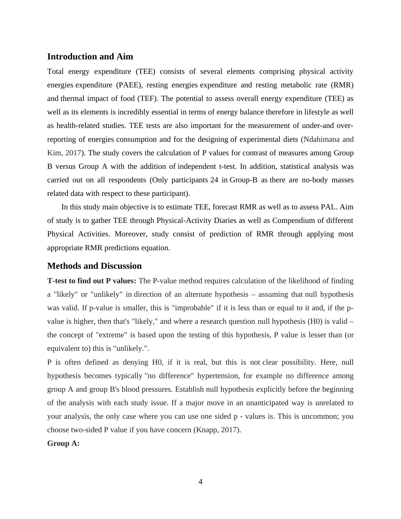
Introduction and Aim
Total energy expenditure (TEE) consists of several elements comprising physical activity
energies expenditure (PAEE), resting energies expenditure and resting metabolic rate (RMR)
and thermal impact of food (TEF). The potential to assess overall energy expenditure (TEE) as
well as its elements is incredibly essential in terms of energy balance therefore in lifestyle as well
as health-related studies. TEE tests are also important for the measurement of under-and over-
reporting of energies consumption and for the designing of experimental diets (Ndahimana and
Kim, 2017). The study covers the calculation of P values for contrast of measures among Group
B versus Group A with the addition of independent t-test. In addition, statistical analysis was
carried out on all respondents (Only participants 24 in Group-B as there are no-body masses
related data with respect to these participant).
In this study main objective is to estimate TEE, forecast RMR as well as to assess PAL. Aim
of study is to gather TEE through Physical-Activity Diaries as well as Compendium of different
Physical Activities. Moreover, study consist of prediction of RMR through applying most
appropriate RMR predictions equation.
Methods and Discussion
T-test to find out P values: The P-value method requires calculation of the likelihood of finding
a "likely" or "unlikely" in direction of an alternate hypothesis – assuming that null hypothesis
was valid. If p-value is smaller, this is "improbable" if it is less than or equal to it and, if the p-
value is higher, then that's "likely," and where a research question null hypothesis (H0) is valid –
the concept of "extreme" is based upon the testing of this hypothesis, P value is lesser than (or
equivalent to) this is "unlikely.".
P is often defined as denying H0, if it is real, but this is not clear possibility. Here, null
hypothesis becomes typically "no difference" hypertension, for example no difference among
group A and group B's blood pressures. Establish null hypothesis explicitly before the beginning
of the analysis with each study issue. If a major move in an unanticipated way is unrelated to
your analysis, the only case where you can use one sided p - values is. This is uncommon; you
choose two-sided P value if you have concern (Knapp, 2017).
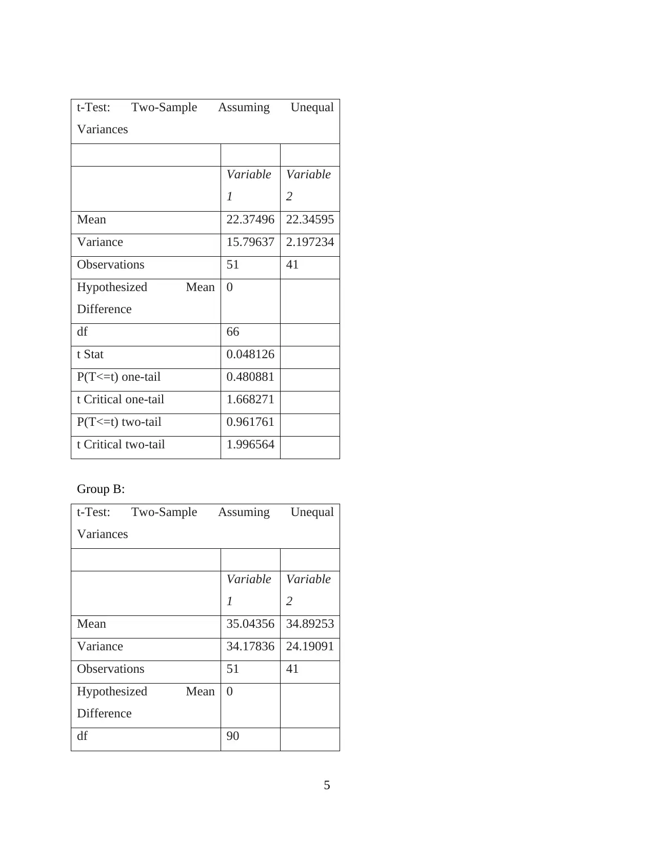
Group A:
4

t-Test: Two-Sample Assuming Unequal
Variances
Variable
1
Variable
2
Mean 22.37496 22.34595
Variance 15.79637 2.197234
Observations 51 41
Hypothesized Mean
Difference
0
df 66
t Stat 0.048126
P(T<=t) one-tail 0.480881
t Critical one-tail 1.668271
P(T<=t) two-tail 0.961761
t Critical two-tail 1.996564
Group B:
t-Test: Two-Sample Assuming Unequal
Variances
Variable
1
Variable
2
Mean 35.04356 34.89253
Variance 34.17836 24.19091
Observations 51 41
Hypothesized Mean
Difference
0
df 90
5

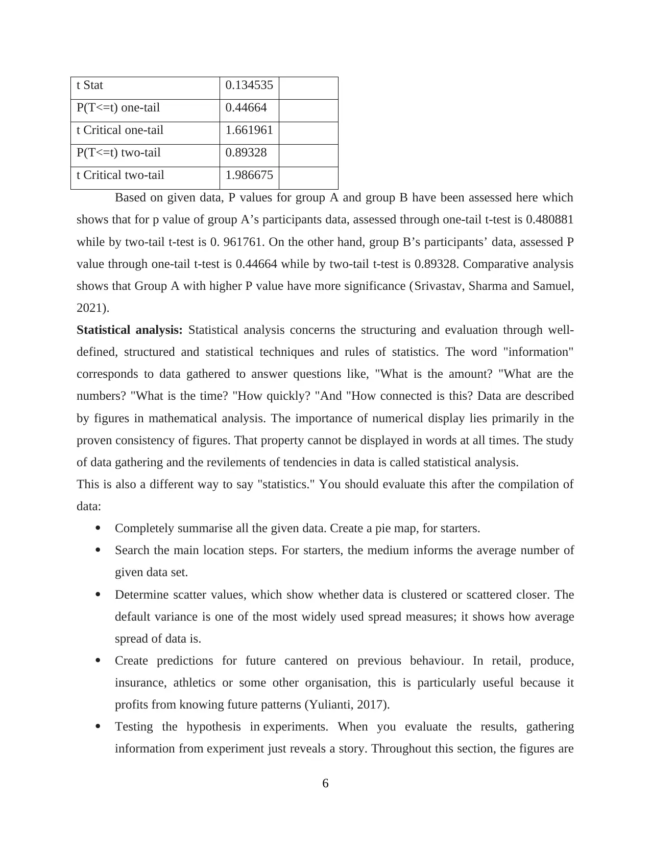
t Stat 0.134535
P(T<=t) one-tail 0.44664
t Critical one-tail 1.661961
P(T<=t) two-tail 0.89328
t Critical two-tail 1.986675
Based on given data, P values for group A and group B have been assessed here which
shows that for p value of group A’s participants data, assessed through one-tail t-test is 0.480881
while by two-tail t-test is 0. 961761. On the other hand, group B’s participants’ data, assessed P
value through one-tail t-test is 0.44664 while by two-tail t-test is 0.89328. Comparative analysis
shows that Group A with higher P value have more significance (Srivastav, Sharma and Samuel,
2021).
Statistical analysis: Statistical analysis concerns the structuring and evaluation through well-
defined, structured and statistical techniques and rules of statistics. The word "information"
corresponds to data gathered to answer questions like, "What is the amount? "What are the
numbers? "What is the time? "How quickly? "And "How connected is this? Data are described
by figures in mathematical analysis. The importance of numerical display lies primarily in the
proven consistency of figures. That property cannot be displayed in words at all times. The study
of data gathering and the revilements of tendencies in data is called statistical analysis.
This is also a different way to say "statistics." You should evaluate this after the compilation of
data:
 Completely summarise all the given data. Create a pie map, for starters.
 Search the main location steps. For starters, the medium informs the average number of
given data set.
 Determine scatter values, which show whether data is clustered or scattered closer. The
default variance is one of the most widely used spread measures; it shows how average
spread of data is.
 Create predictions for future cantered on previous behaviour. In retail, produce,
insurance, athletics or some other organisation, this is particularly useful because it
profits from knowing future patterns (Yulianti, 2017).
 Testing the hypothesis in experiments. When you evaluate the results, gathering
information from experiment just reveals a story. Throughout this section, the figures are
6

officially referred to as "Hypothesis Testing," which either demonstrates or refutes null
hypothesis (the popular theory).
 Statistical analysis in study is primarily employed for extensively for scientific study,
from common physics to critical social sciences. Along with test hypotheses,
certain statistics may provide an estimate for an uncertainty that is challenging or hard to
calculate. For instance, field of quantum ground theory whilst also offering success
on theoretical side of factors has proven problematic for empirical experiments and
evaluation. A few other social science subjects, such as report of consciousness as well as
selection, are virtually unfeasible to quantify data analysis can cast doubt on what is most
likely or slightest probable option (Guetterman, 2019).
In this regard following is comprehensive statistical analysis of given data, as follows:
For Group A:
Variable
1
Variable
2
Mean 22.37496 22.34595
Variance 15.79637 2.197234
Observations 51 41
For Group B:
Variable
1
Variable
2
Mean 35.04356 34.89253
Variance 34.17836 24.19091
Observations 51 41
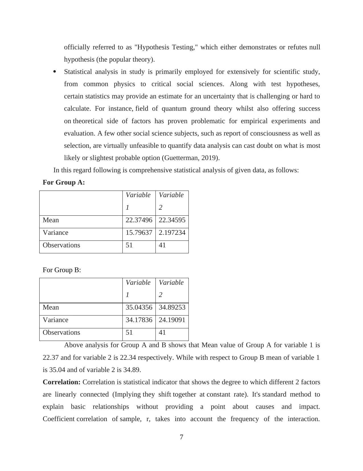
Above analysis for Group A and B shows that Mean value of Group A for variable 1 is
22.37 and for variable 2 is 22.34 respectively. While with respect to Group B mean of variable 1
is 35.04 and of variable 2 is 34.89.
Correlation: Correlation is statistical indicator that shows the degree to which different 2 factors
are linearly connected (Implying they shift together at constant rate). It's standard method to
explain basic relationships without providing a point about causes and impact.
Coefficient correlation of sample, r, takes into account the frequency of the interaction.
7

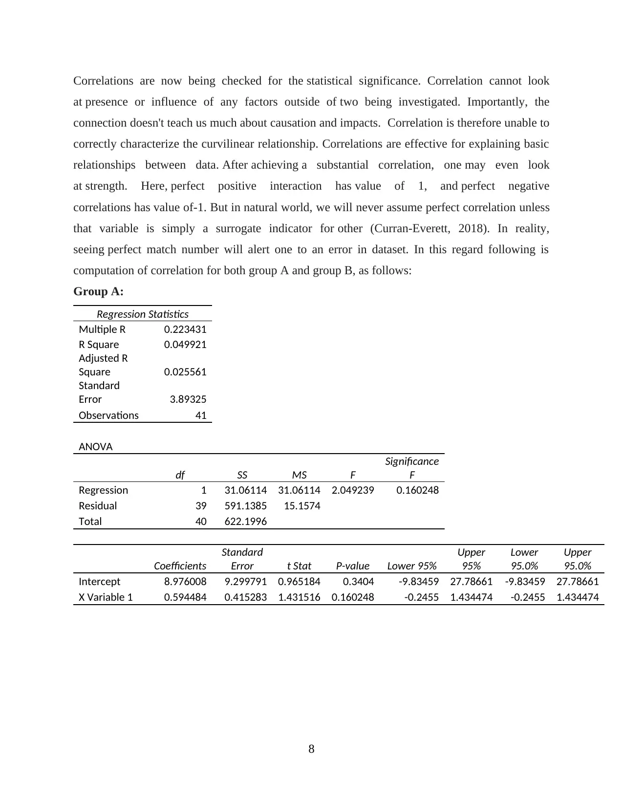
Correlations are now being checked for the statistical significance. Correlation cannot look
at presence or influence of any factors outside of two being investigated. Importantly, the
connection doesn't teach us much about causation and impacts. Correlation is therefore unable to
correctly characterize the curvilinear relationship. Correlations are effective for explaining basic
relationships between data. After achieving a substantial correlation, one may even look
at strength. Here, perfect positive interaction has value of 1, and perfect negative
correlations has value of-1. But in natural world, we will never assume perfect correlation unless
that variable is simply a surrogate indicator for other (Curran-Everett, 2018). In reality,
seeing perfect match number will alert one to an error in dataset. In this regard following is
computation of correlation for both group A and group B, as follows:
Group A:
Regression Statistics
Multiple R 0.223431
R Square 0.049921
Adjusted R
Square 0.025561
Standard
Error 3.89325
Observations 41
ANOVA
df SS MS F
Significance
F
Regression 1 31.06114 31.06114 2.049239 0.160248
Residual 39 591.1385 15.1574
Total 40 622.1996
Coefficients
Standard
Error t Stat P-value Lower 95%
Upper
95%
Lower
95.0%
Upper
95.0%
Intercept 8.976008 9.299791 0.965184 0.3404 -9.83459 27.78661 -9.83459 27.78661
X Variable 1 0.594484 0.415283 1.431516 0.160248 -0.2455 1.434474 -0.2455 1.434474
8

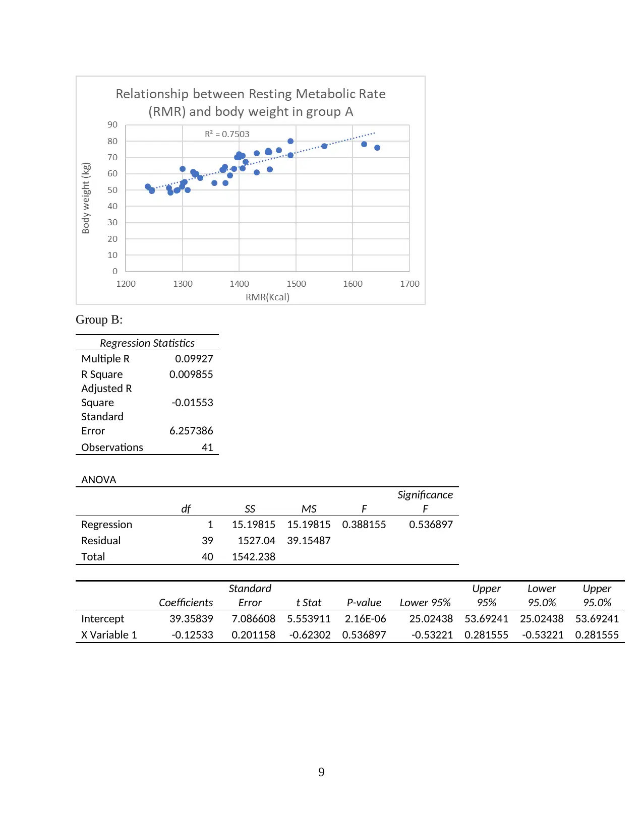
Group B:
Regression Statistics
Multiple R 0.09927
R Square 0.009855
Adjusted R
Square -0.01553
Standard
Error 6.257386
Observations 41
ANOVA
df SS MS F
Significance
F
Regression 1 15.19815 15.19815 0.388155 0.536897
Residual 39 1527.04 39.15487
Total 40 1542.238
Coefficients
Standard
Error t Stat P-value Lower 95%
Upper
95%
Lower
95.0%
Upper
95.0%
Intercept 39.35839 7.086608 5.553911 2.16E-06 25.02438 53.69241 25.02438 53.69241
X Variable 1 -0.12533 0.201158 -0.62302 0.536897 -0.53221 0.281555 -0.53221 0.281555
9

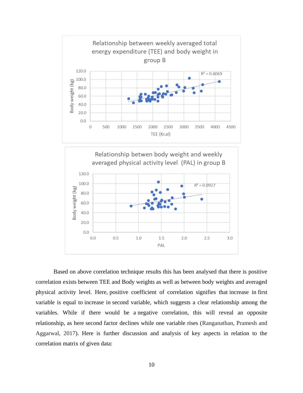
Based on above correlation technique results this has been analysed that there is positive
correlation exists between TEE and Body weights as well as between body weights and averaged
physical activity level. Here, positive coefficient of correlation signifies that increase in first
variable is equal to increase in second variable, which suggests a clear relationship among the
variables. While if there would be a negative correlation, this will reveal an opposite
relationship, as here second factor declines while one variable rises (Ranganathan, Pramesh and
Aggarwal, 2017). Here is further discussion and analysis of key aspects in relation to the
correlation matrix of given data:
10

RMR: Resting metabolic-rate (RMR) is quite widely used because it helps person to sleep at
house to drive to lab in morning, and to relax there until RMR is evaluated. The meanings for
BMR as well as RMR are generally lesser than 10% different and are often used derogatively.
RMR is usually close to around 4.2 kJ per kg weight per hour and 3.5 ml O2 kg-per body weight
per minute. Estimations on RMR are carried out employing indirect mass spectroscopy and a
computerized open-circuit ventilated-hood framework. Participants laid supine with each
assessment carrying out for around 15 minutes and the very first five minutes of data were
eliminated to ensure that only consistent resting variables were collected. Ventilated hood
has cranial opening that enables incursion of the ambient air, caudal opening that is connected
to main body of equipment by hose. The device pulls air through hood at a steady flow rate and
measures fraction of exhausted CO2 (FECO2) and O2 (FEO2) and afterwards measures rate of
oxygen intake (V-cit O2) as well as rate of the carbon dioxide (V-cit CO2). Such values of V-
circulated O2 and V-circulated CO2 are being used to measure high carbohydrate oxidation
rates, energy consumption rates, using indirect calorimetric equations. Despite recognized
drawbacks, RMR prediction algorithms provide a realistic alternative to indirect calorimetric
RMR calculations, as some energy requirements could be measured using regularly available
measurements such as weights, age, gender and height. Expenditure on indirect calorimetry
devices, the need for qualified staff, as well as time-consuming aspect of RMR calculation
prohibits the regular provision of the indirect calorimetry (Heydenreich, Kayser, Schutz and
Melzer, 2017).
Metabolic equivalents (MET): One MET being equal to the amount of oxygen intake (V to O2)
at rests or in quiet sitting posture and is comparable to 3.5 ml/min/kg of body mass or 1
kcal/hour/kg body mass. The MET of given activity is ratio of metabolic rate of an activity
to resting metabolic rate which indicates how often times the energy consumption of given
activity is greater than that of energy expenditure at idle. Thorough MET estimates and therefore
EE averages for various physical activities are being formulated in the Physical Activity
Compilation, with functions starting from 0.9 MET (going to sleep) to 18 the MET (sleeping).
Actual energy costs can vary between people due to variations in body weight, dyslipidaemia,
age and sex. In order to account for variations in body mass, METs are represented as EE levels
per kg body mass. Use of Physical Activities Compendium allows the calculation of daily EAs
through physical activity journals, offering information about the nature, severity and length
11

within each activity used in the normal lifestyle. A complete set of the energy costs of the
various athletic exercises will be submitted to Moodle (Zusman and et.al., 2019).
Conclusion
From above study-report, this has been articulated that scientific report provides
comprehensive details regarding each aspect of data selected. The study helps researchers and
analysts to thoroughly analyse each and every variable as well as to assess the key relation
among different variables.
12

REFERENCES
Books and Journals:
Ndahimana, D. and Kim, E.K., 2017. Measurement methods for physical activity and energy
expenditure: a review. Clinical nutrition research, 6(2), p.68.
Knapp, A.C., 2017. The Effect of Aerobic Exercise Training on Components of Total Energy
Expenditure (Doctoral dissertation, University of South Alabama).
Yulianti, D., 2017, March. Problem-based learning model used to scientific approach based
worksheet for physics to develop senior high school students characters. In Journal of
Physics: Conference Series (Vol. 824, No. 1, p. 012009). IOP Publishing.
Guetterman, T.C., 2019. Basics of statistics for primary care research. Family medicine and
community health, 7(2).
Curran-Everett, D., 2018. Explorations in statistics: the log transformation. Advances in
physiology education, 42(2), pp.343-347.
Ranganathan, P., Pramesh, C.S. and Aggarwal, R., 2017. Common pitfalls in statistical analysis:
Measures of agreement. Perspectives in clinical research, 8(4), p.187.
Heydenreich, J., Kayser, B., Schutz, Y. and Melzer, K., 2017. Total energy expenditure, energy
intake, and body composition in endurance athletes across the training season: A
systematic review. Sports medicine-open, 3(1), pp.1-24.
Zusman, O. and et.al., 2019. Predictive equations versus measured energy expenditure by
indirect calorimetry: a retrospective validation. Clinical nutrition, 38(3), pp.1206-1210.
Srivastav, A.K., Sharma, N. and Samuel, A.J., 2021. Impact of Coronavirus disease-19 (COVID-
19) lockdown on physical activity and energy expenditure among physiotherapy
professionals and students using web-based open E-survey sent through WhatsApp,
Facebook and Instagram messengers. Clinical Epidemiology and Global Health, 9,
pp.78-84.
13

Appendix
Group A
RESIDUAL OUTPUT
Observation
Predicted
Y Residuals
1 22.38708 -5.38028
2 23.56403 2.000928
3 22.84712 -1.04781
4 23.34379 2.046839
5 23.14811 -2.35138
6 22.57982 6.852313
7 21.93394 -1.36514
8 22.82638 1.741092
9 20.71003 -1.34019
10 22.4253 -3.19761
11 23.05839 -0.82933
12 22.46909 0.915262
13 22.43678 -3.75166
14 23.26341 -2.22615
15 21.42943 0.05495
16 23.74347 -7.22874
17 21.38408 -0.62283
18 22.90095 1.584704
19 21.03924 -4.08422
20 22.3787 -3.34756
21 23.06246 6.698379
22 23.04093 -0.94064
23 20.78759 -1.6875
24 21.7682 3.735836
25 21.13341 0.170539
26 22.90008 -2.15253
27 21.91479 -3.36564
28 22.27851 -4.21235
29 22.79313 -1.56255
30 22.16035 0.523959
31 21.58566 -3.37901
32 22.16842 -1.7532
33 21.12114 -1.83176
34 22.60878 1.186577
35 22.81988 0.234679
14

36 21.58558 4.691706
37 20.82456 5.154124
38 20.56381 -1.81381
39 21.12114 9.738236
40 23.12253 10.60808
41 23.44334 1.5337
Group B
RESIDUAL OUTPUT
Observation
Predicted
Y Residuals
1 35.76397 4.218173
2 34.95477 2.50026
3 35.61455 5.825359
4 35.85078 -10.82
5 34.25024 -6.23054
6 34.51522 -4.82404
7 35.42199 -0.73243
8 34.77245 0.082682
9 34.17639 -2.93591
10 35.15678 2.57834
11 34.15195 3.153544
12 34.10864 -0.58916
13 33.22294 -10.4134
14 34.3912 15.0076
15 34.31504 -0.60595
16 35.12424 -2.91686
17 35.04525 3.429755
18 36.50262 -1.8528
19 35.12294 -2.97033
20 35.03821 -5.9473
21 35.4224 -8.00932
22 35.89367 -1.69416
23 35.31094 4.576418
24 34.74163 8.834315
25 35.3059 4.726123
26 35.36494 -8.18672
27 34.79368 6.432436
28 34.77654 -2.00571
29 35.01368 2.670958
30 35.6137 -7.27603
15

31 35.28554 0.885036
32 35.62229 -8.62793
33 35.30868 -3.58488
34 34.48007 -0.50173
35 34.50872 -4.24164
36 34.73609 6.178325
37 34.99283 -3.03716
38 35.64599 9.543295
39 34.94171 6.796087
40 34.24227 -3.49895
41 34.90289 14.06425
16