ELE4605 - Numerical Modeling of TEM Waves in Transmission Lines

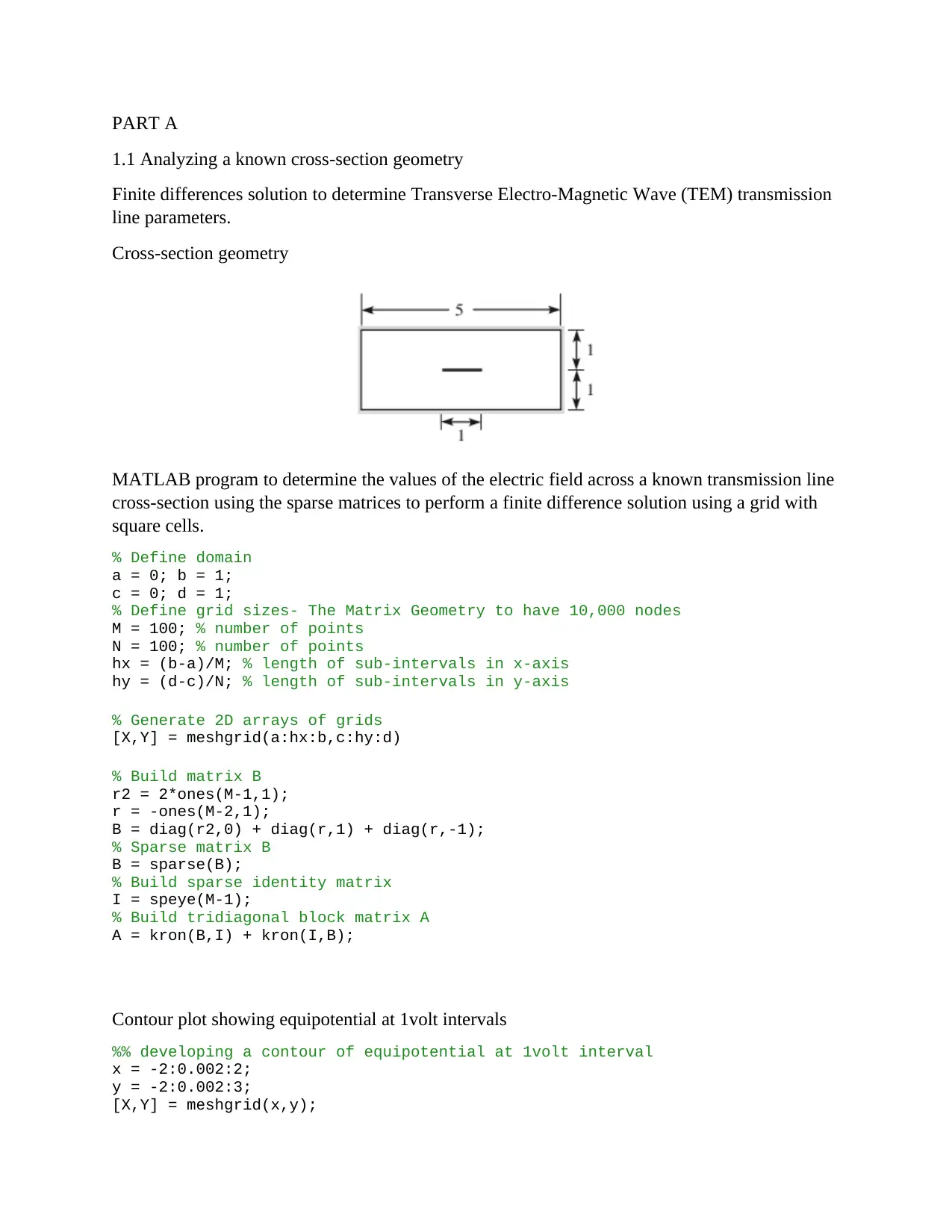
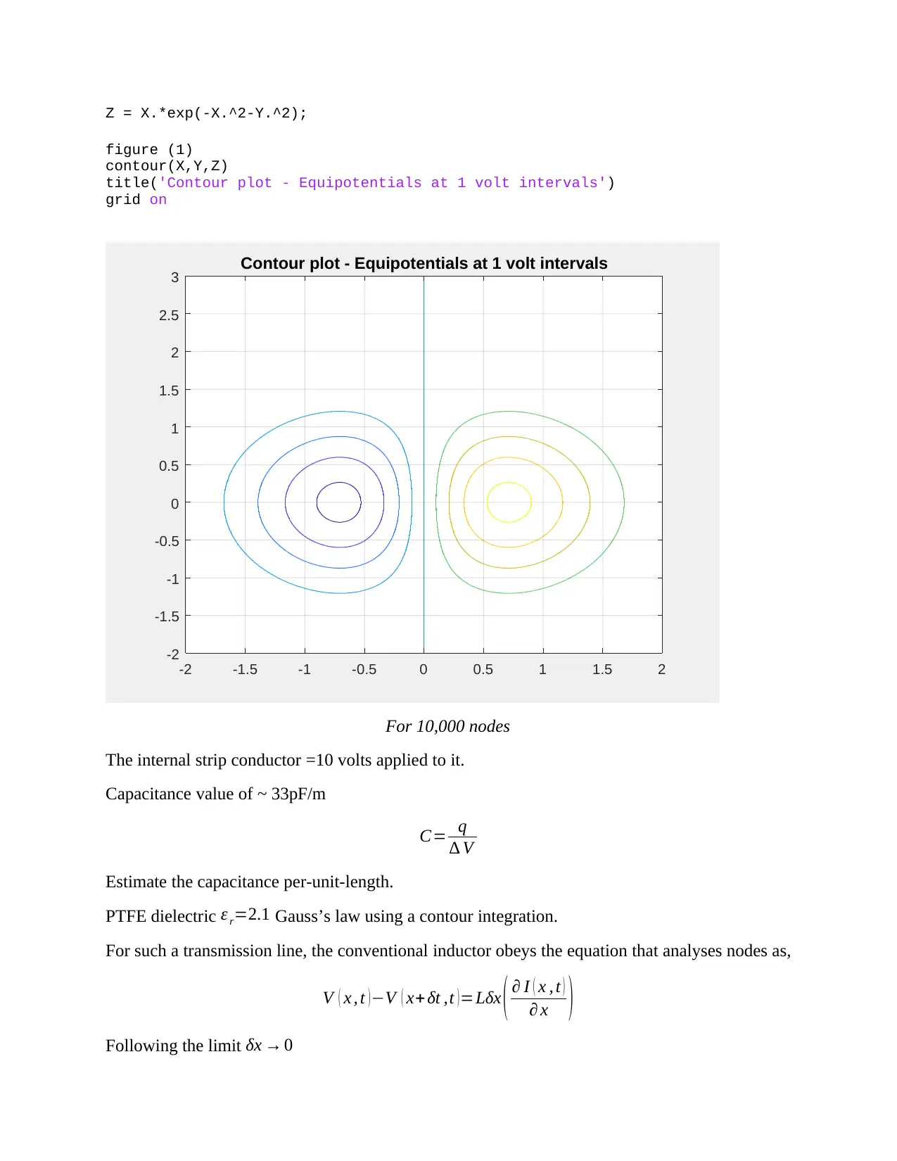
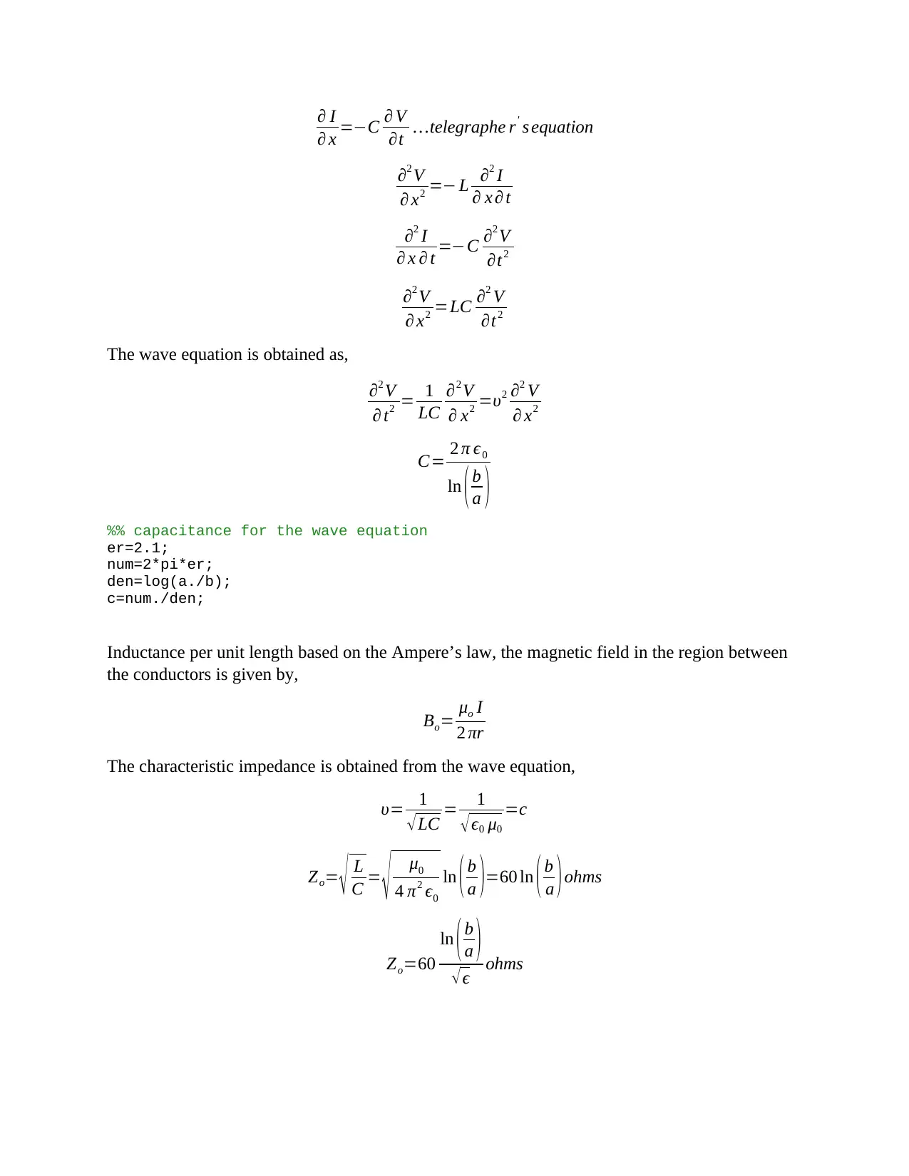
This assignment focuses on analyzing Transverse Electro-Magnetic (TEM) wave transmission line parameters using the finite difference method implemented in MATLAB. The program calculates the electric field across a known transmission line cross-section using sparse matrices and a ...Read More

UNIVERSITY AFFILIATION
FACULTY OR DEPARTMENT
SCHOOL ID & NAME
TITLE:
STUDENT NAME
STUDENT NUMBER
PROFESSOR (TUTOR)
DATE OF SUBMISSION
2018

PART A
1.1 Analyzing a known cross-section geometry
Finite differences solution to determine Transverse Electro-Magnetic Wave (TEM) transmission
line parameters.
Cross-section geometry
MATLAB program to determine the values of the electric field across a known transmission line
cross-section using the sparse matrices to perform a finite difference solution using a grid with
square cells.
% Define domain
a = 0; b = 1;
c = 0; d = 1;
% Define grid sizes- The Matrix Geometry to have 10,000 nodes
M = 100; % number of points
N = 100; % number of points
hx = (b-a)/M; % length of sub-intervals in x-axis
hy = (d-c)/N; % length of sub-intervals in y-axis
% Generate 2D arrays of grids
[X,Y] = meshgrid(a:hx:b,c:hy:d)
% Build matrix B
r2 = 2*ones(M-1,1);
r = -ones(M-2,1);
B = diag(r2,0) + diag(r,1) + diag(r,-1);
% Sparse matrix B
B = sparse(B);
% Build sparse identity matrix
I = speye(M-1);
% Build tridiagonal block matrix A
A = kron(B,I) + kron(I,B);
Contour plot showing equipotential at 1volt intervals
%% developing a contour of equipotential at 1volt interval
x = -2:0.002:2;
y = -2:0.002:3;
[X,Y] = meshgrid(x,y);

Z = X.*exp(-X.^2-Y.^2);
figure (1)
contour(X,Y,Z)
title('Contour plot - Equipotentials at 1 volt intervals')
grid on
Contour plot - Equipotentials at 1 volt intervals
-2 -1.5 -1 -0.5 0 0.5 1 1.5 2
-2
-1.5
-1
-0.5
0
0.5
1
1.5
2
2.5
3
For 10,000 nodes
The internal strip conductor =10 volts applied to it.
Capacitance value of ~ 33pF/m
C= q
∆ V
Estimate the capacitance per-unit-length.
PTFE dielectric ε r=2.1 Gauss’s law using a contour integration.
For such a transmission line, the conventional inductor obeys the equation that analyses nodes as,
V ( x , t )−V ( x+ δt ,t )=Lδx ( ∂ I ( x , t )
∂ x )
Following the limit δx → 0

∂ I
∂ x =−C ∂ V
∂t …telegraphe r' s equation
∂2 V
∂ x2 =− L ∂2 I
∂ x ∂ t
∂2 I
∂ x ∂ t =−C ∂2 V
∂t2
∂2 V
∂ x2 =LC ∂2 V
∂t2
The wave equation is obtained as,
∂2 V
∂ t2 = 1
LC
∂2 V
∂ x2 =υ2 ∂2 V
∂ x2
C= 2 π ϵ0
ln ( b
a )
%% capacitance for the wave equation
er=2.1;
num=2*pi*er;
den=log(a./b);
c=num./den;
Inductance per unit length based on the Ampere’s law, the magnetic field in the region between
the conductors is given by,
Bo= μo I
2 πr
The characteristic impedance is obtained from the wave equation,
υ= 1
√LC = 1
√ϵ0 μ0
=c
Zo= √ L
C = √ μ0
4 π2 ϵ0
ln ( b
a )=60 ln ( b
a ) ohms
Zo=60
ln ( b
a )
√ ϵ ohms

1.2 Applying your program to an unknown geometry
PART B
Based on my student number, the transmission line cross-section used is,
Coupled-channel line, type 2, unbalanced.
In the unbalanced mode, the conductors are at the same voltage with respect to the ground. The
cross section has symmetry of about the vertical axis and the comparable nodes on either side of
the axis will have the same voltages. The integration contour should close both conductors and is
best positioned against the shield so that the outer summation is zero.
Solution