Numeracy & Data Analysis: Forecasting Scotland Temperature Trends

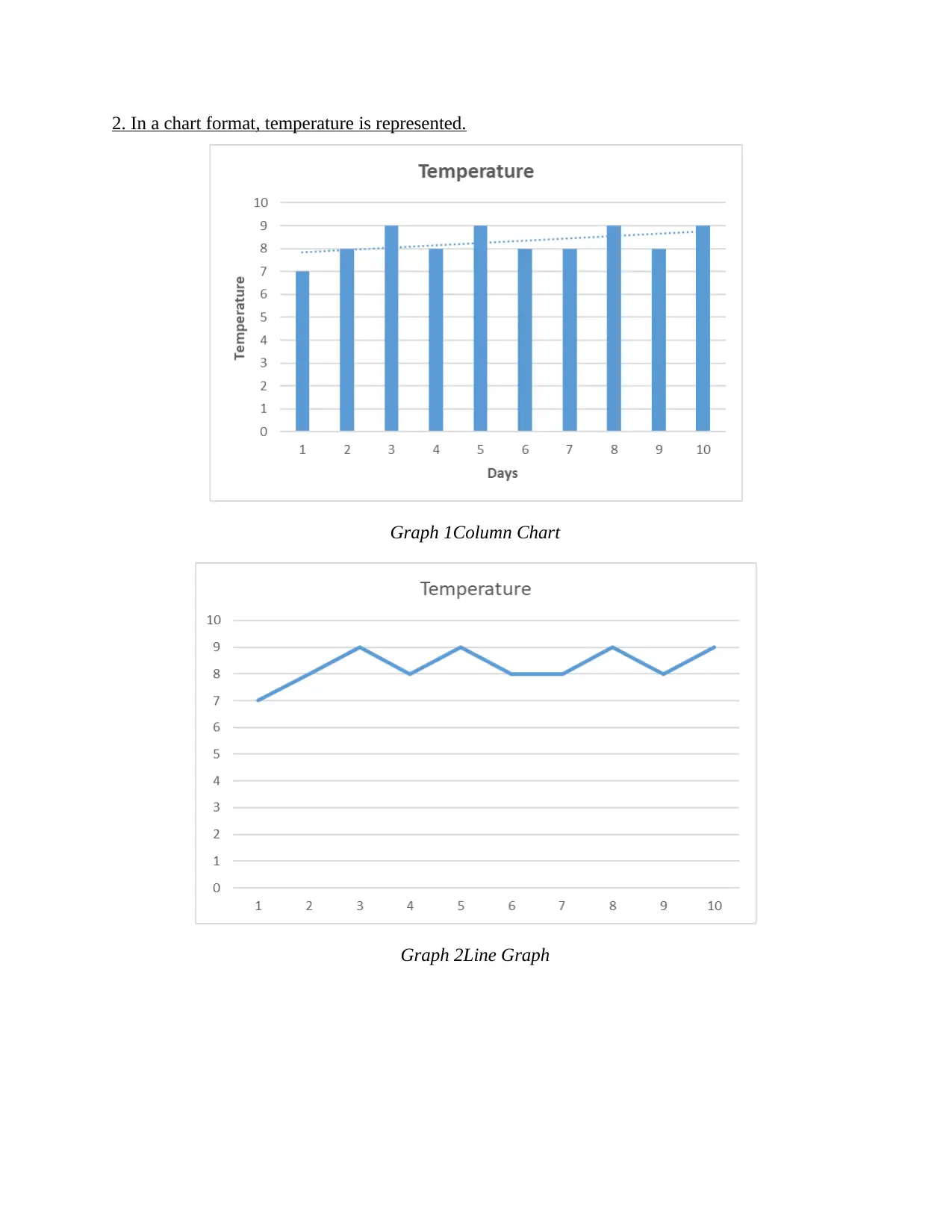
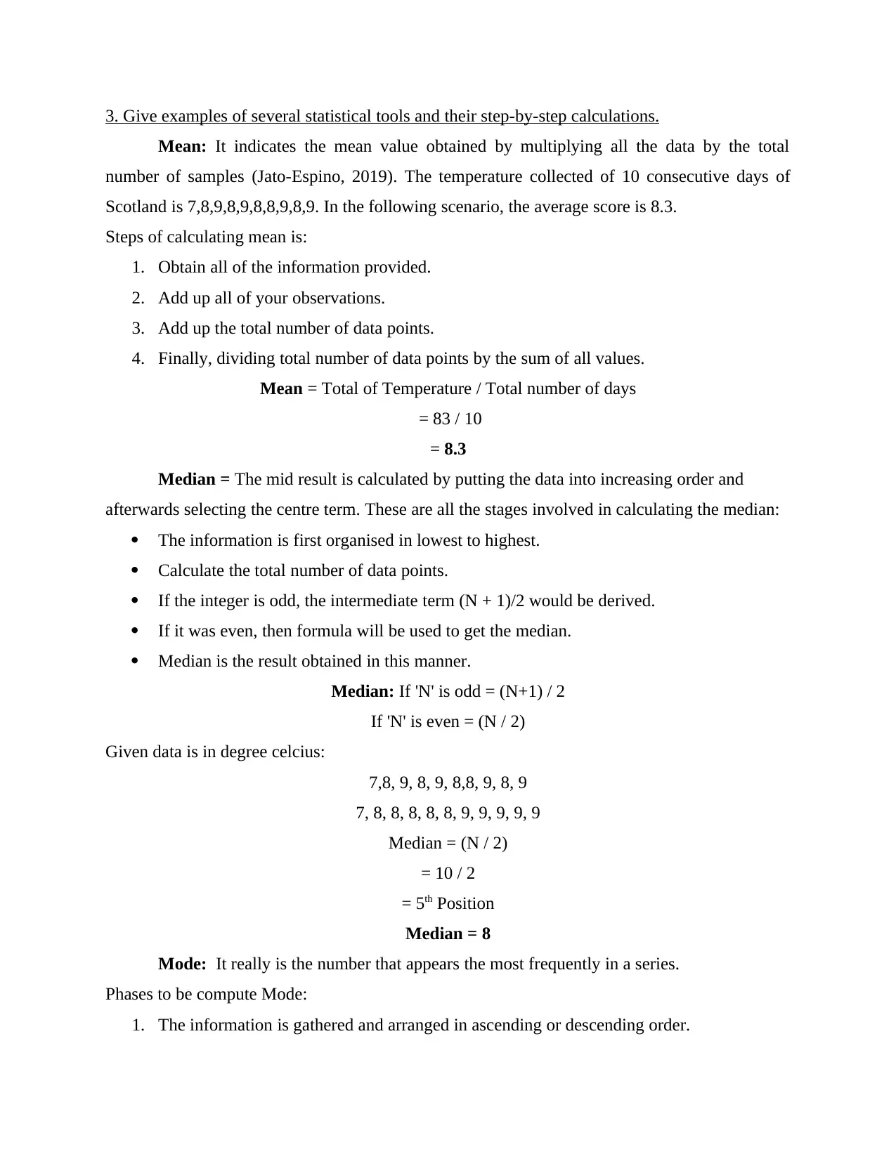
This report provides a detailed analysis of temperature variations in Scotland over a ten-day period. It uses statistical tools such as mean, median, mode, range, and standard deviation to describe the temperature data. The report includes column and line graphs to visually represent the temperature trends. Furthermore, it applies the Linear Forecasting Model to predict future temperatures, calculating the values of 'm' and 'c' and forecasting the temperature for the 12th and 14th days. The analysis concludes that the temperature in Scotland varied between 7, 8, and 9 degrees Celsius during the observed period, with the forecasting model providing predictions for subsequent days.

Numeracy and Data
Analysis

Contents
INTRODUCTION...........................................................................................................................3
MAIN BODY..................................................................................................................................3
1. Compile the information into a table.......................................................................................3
2. In a chart format, temperature is represented..........................................................................4
3. Give examples of several statistical tools and their step-by-step calculations........................5
4. Perform regression analysis and discover the values of m and c using the Linear Forecasting
model...........................................................................................................................................7
CONCLUSION................................................................................................................................8
REFERENCES................................................................................................................................9

INTRODUCTION
The concept of numeracy refers to the use of mathematics in everyday life. Graphics are
often used to depict unstructured data in a systematic and useful manner (Ramli and et.al., 2019).
The report mainly uses data from the previous ten days to examine temperature variations in
Scotland. The Linear Forecasting Model is being used to anticipate the temperature of another
few days.
MAIN BODY
1. Compile the information into a table.
Day
Temperatu
re
1 7
2 8
3 9
4 8
5 9
6 8
7 8
8 9
9 8
10 9

2. In a chart format, temperature is represented.
Graph 1Column Chart
Graph 2Line Graph

3. Give examples of several statistical tools and their step-by-step calculations.
Mean: It indicates the mean value obtained by multiplying all the data by the total
number of samples (Jato-Espino, 2019). The temperature collected of 10 consecutive days of
Scotland is 7,8,9,8,9,8,8,9,8,9. In the following scenario, the average score is 8.3.
Steps of calculating mean is:
1. Obtain all of the information provided.
2. Add up all of your observations.
3. Add up the total number of data points.
4. Finally, dividing total number of data points by the sum of all values.
Mean = Total of Temperature / Total number of days
= 83 / 10
= 8.3
Median = The mid result is calculated by putting the data into increasing order and
afterwards selecting the centre term. These are all the stages involved in calculating the median:
 The information is first organised in lowest to highest.
 Calculate the total number of data points.
 If the integer is odd, the intermediate term (N + 1)/2 would be derived.
 If it was even, then formula will be used to get the median.
 Median is the result obtained in this manner.
Median: If 'N' is odd = (N+1) / 2
If 'N' is even = (N / 2)
Given data is in degree celcius:
7,8, 9, 8, 9, 8,8, 9, 8, 9
7, 8, 8, 8, 8, 8, 9, 9, 9, 9, 9
Median = (N / 2)
= 10 / 2
= 5th Position
Median = 8
Mode: It really is the number that appears the most frequently in a series.
Phases to be compute Mode:
1. The information is gathered and arranged in ascending or descending order.

2. Obtain the value that has appeared the most times.
3. Count how many times the number has appeared.
4. The value which has most number of frequencies is termed as mode.
Mode = 8
Range: It is the result of deducting the minimum number first from greatest value in a
group of statistics. If indeed the range is broad, this is not part of the main tendency; but, if the
range is tiny, it is responsibility of the central tendency.
Steps of computing Range:
1. Sort the data that has been provided.
2. Determine the lowest and highest figure based on the information provided.
3. The least value is deducted from the greatest.
4. The Ranges is the result of this calculation.
Range = Highest Value – Lowest Value
Range = 9 - 7
Range = 2
Standard Deviation: It is the statistic that really is determined by measuring the degree
of departure from the average into account (Abbas, 2020).
The procedures to determine Standard Deviation are as follows:
1. To start, calculate the database's Mean.
2. After subtracting the mean value from each data, the change is measured.
3. The totalled valuation obtained.
4. Subtract the total from the set of measurements.
5. Finally, the information's square root is determined.
Standard Deviation= √ (xi – μ)2 / N
= √ (4.1) / 10
= √ 0.41
= 0.64

4. Perform regression analysis and discover the values of m and c using the Linear Forecasting
model.
Linear Forecasting Model: - This model aids in forecasting future values based on statistics of
historical data (Liu and et.al., 2018).
1. Multiply the factors X and Y, which have been the day and temperature respectively.
2. Add up all of above figures.
3. Add the x factor and the y variable separately.
4. Finally, multiply both elements.
5. Substitute the numbers in the equation for ( x)⅀ 2.
6. The value of 'm' is the derived value.
y = mx + c
where, 'y' is the Dependent Factor
'mx' is the Independent Factor
'c' is the constant
m = [10 * 465 – (55) * (83)] / [10 * (385) – (55)2]
m = [4650 – 4565] / [3850 – 3025]
m= 85/ 825
m= 0.103
Steps of calculation value of 'c'
1. Compound the factors X and Y, which have been the date and temperature, respectively.
2. Add up all of the above-mentioned figures.
3. Finally, multiply it by the total of 'N'.
4. The result of 'c' is indeed the value generated from Step 3.

c = 83 – (0.103) * (55) / 10
c = (83 + 5.665) / 10
= 88.665 / 10
= 8.867
Temperature on Day 12: -
m= 0.103, c = 8.867, x= 12,
y = mx + c
y= 0.103 (12) + 8.867
y = 1.236 + 8.867
y = 10.103
Temperature on Day 14: -
m= 0.103, c = 8.867, x =14
y = mx+ c
y= 0.103 (14) + 8.867
y= 1.442 + 8.867
y= 10.309
CONCLUSION
The above asserted report states that the temperature of the city Scotland is 7, 8 and 9 degrees
Celsius all across the 10 days. So, for this the descriptive statistics is calculated along with the
presented column and line graphs. Further, through the help of linear forecasting model the value
of m and c is computed. The 12 and 14th day value of temperature is computed through the figure
of m and c.

REFERENCES
Books and Journals
Abbas, S., 2020. Climate change and cotton production: an empirical investigation of
Pakistan. Environmental science and pollution research, 27(23), pp.29580-29588.
Jato-Espino, D., 2019. Spatiotemporal statistical analysis of the Urban Heat Island effect in a
Mediterranean region. Sustainable Cities and Society, 46, p.101427.
Liu, K. and et.al., 2018. Exploring the interactive effects of ambient temperature and vehicle
auxiliary loads on electric vehicle energy consumption. Applied Energy, 227, pp.324-
331.
Ramli, M.F. and et.al., 2019. Evidence of climate variability from rainfall and temperature
fluctuations in semi-arid region of the tropics. Atmospheric research, 224, pp.52-64.