AQ019-3-2: Time Series Analysis & Forecasting Methods Report

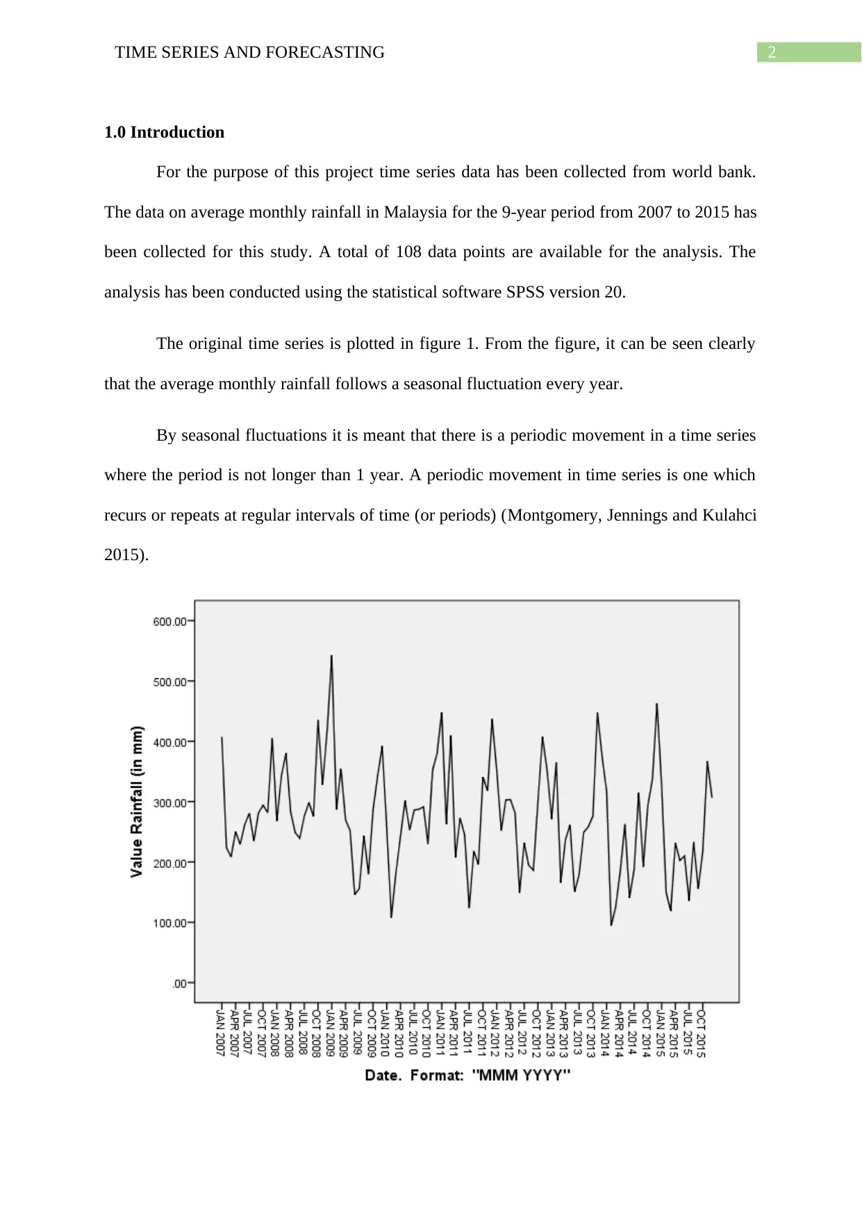
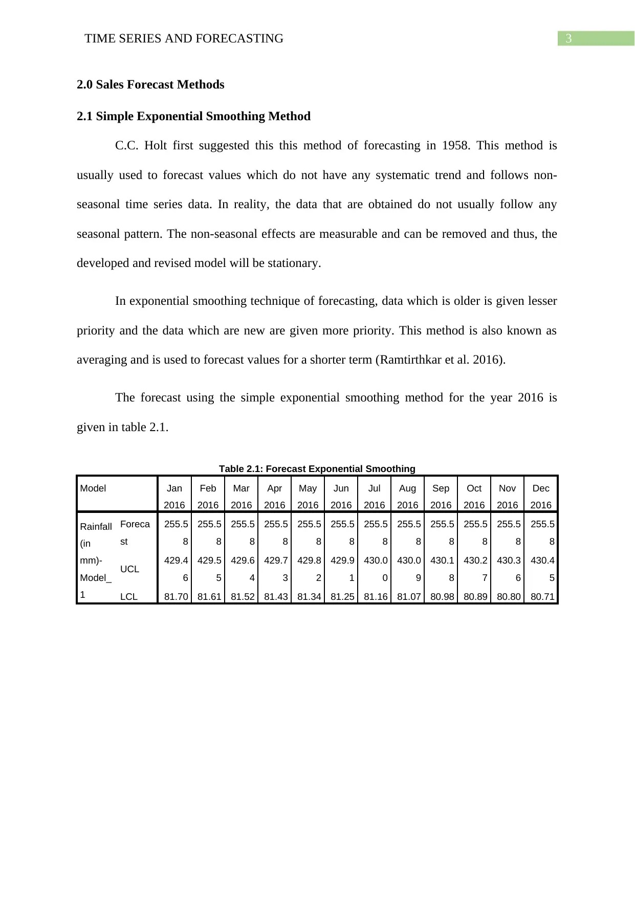
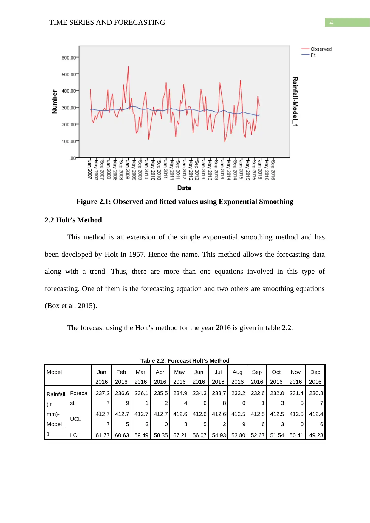
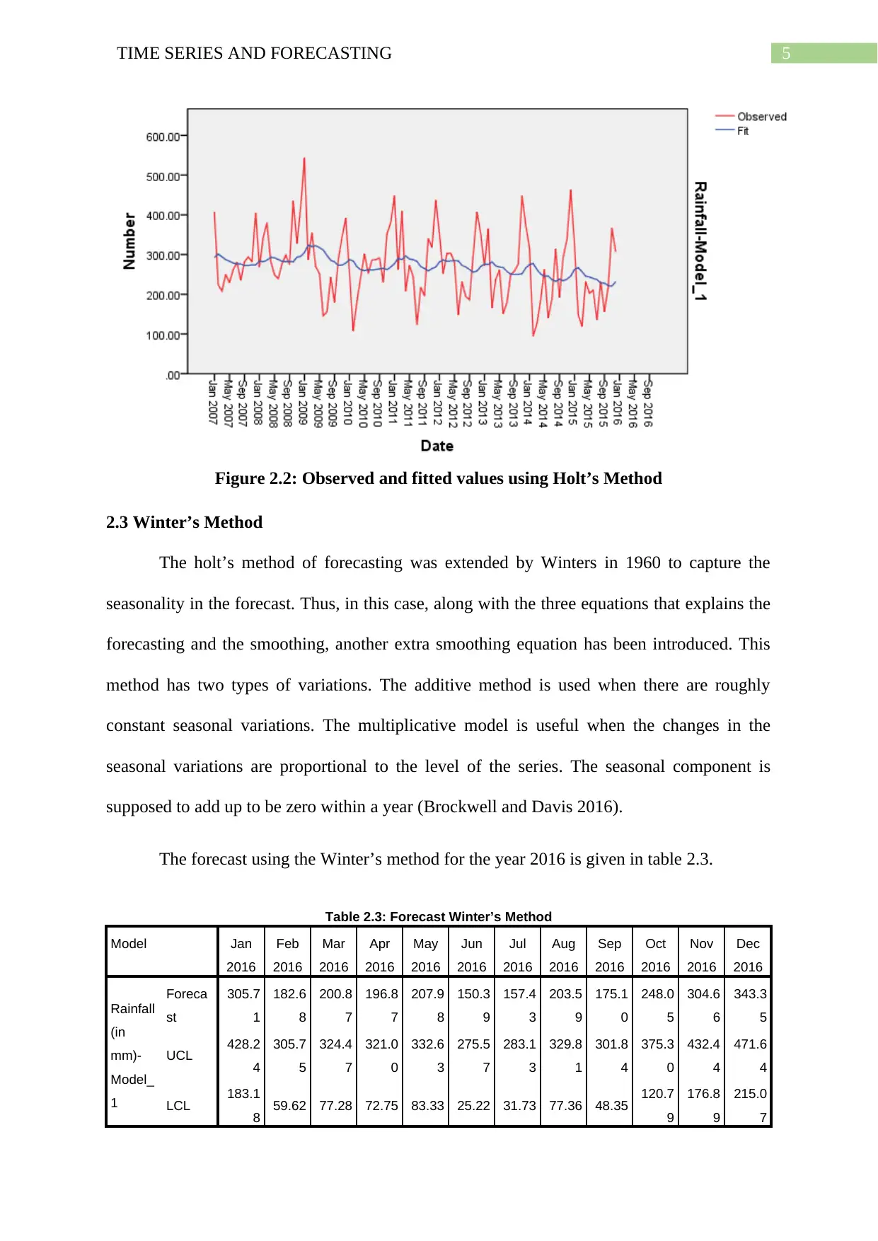
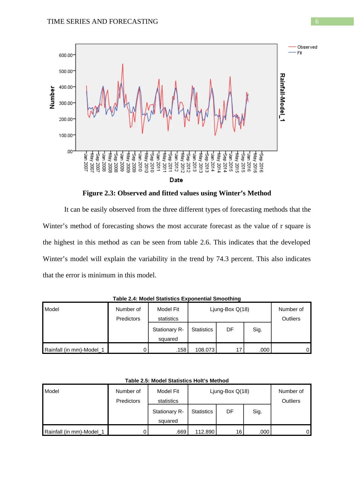
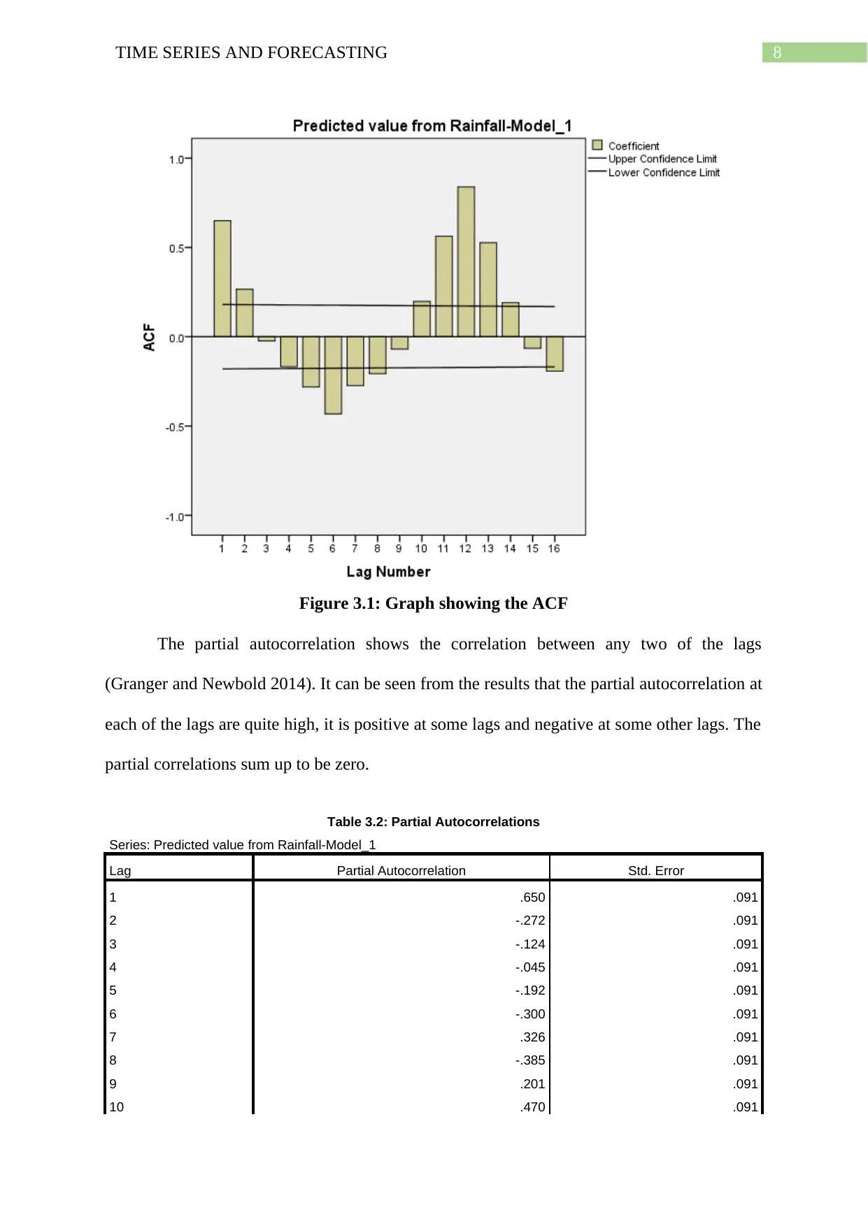
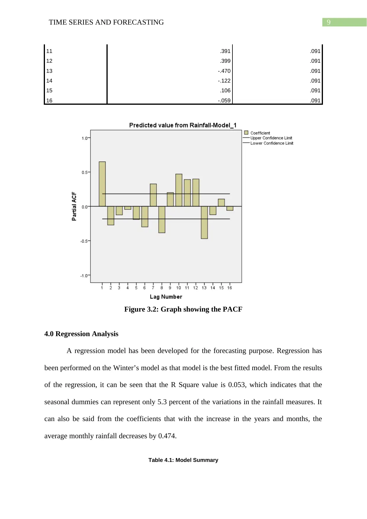
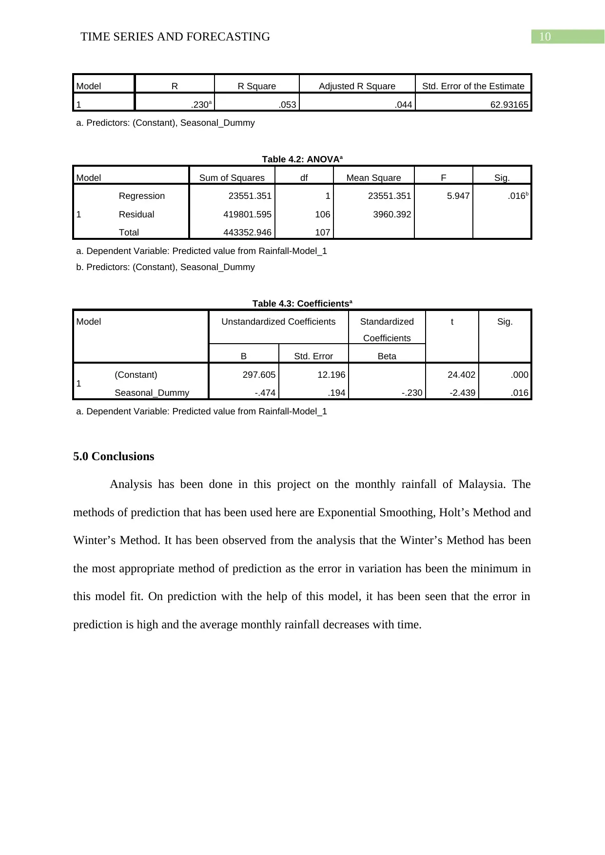
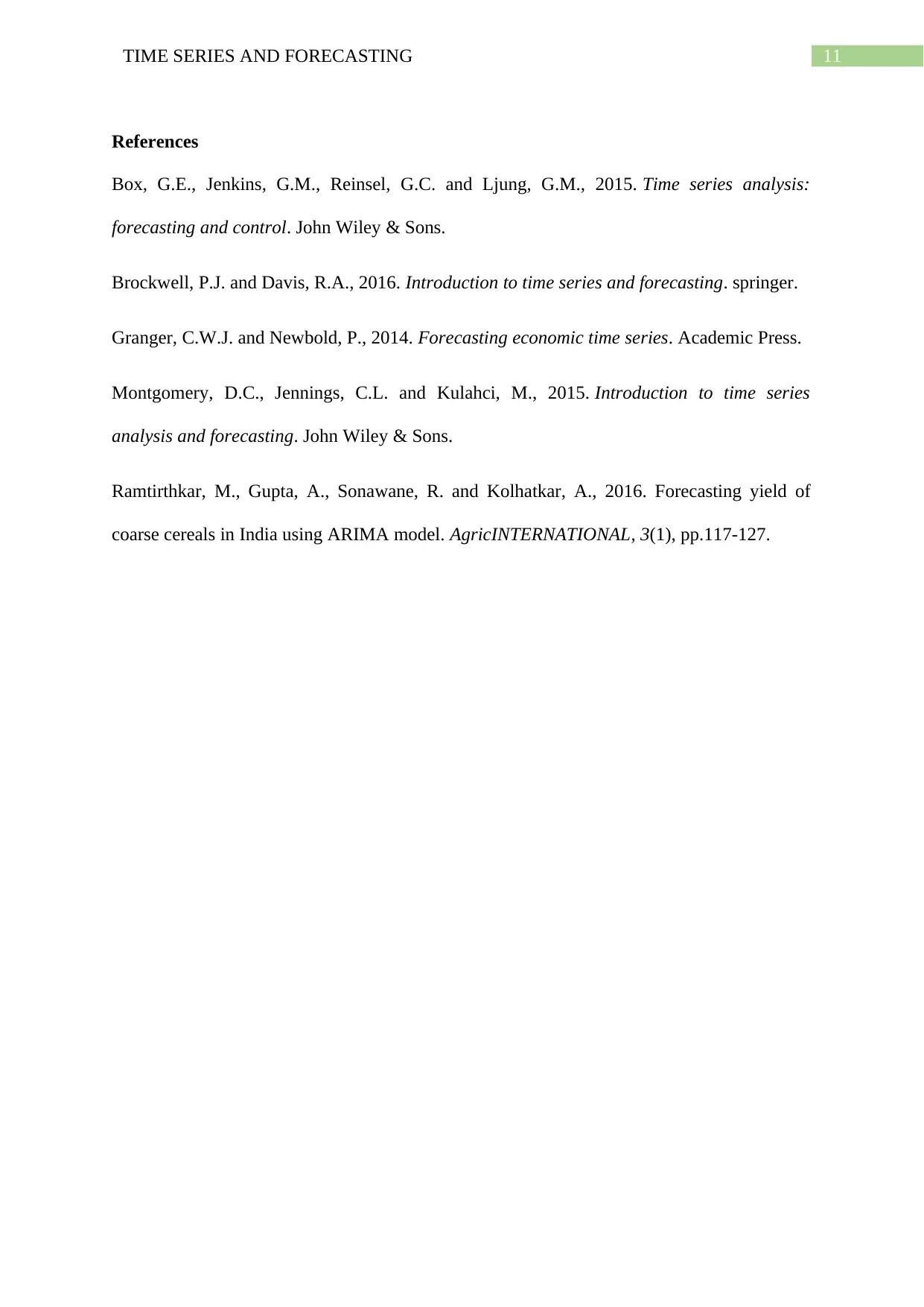
This report presents a time series analysis and forecasting exercise using average monthly rainfall data in Malaysia from 2007 to 2015. The analysis employs three forecasting methods: Simple Exponential Smoothing, Holt's Method, and Winter's Method. Autocorrelation functions (ACF) and partial autocorrelation functions (PACF) are examined to assess the presence of autocorrelation in the developed models. Furthermore, a regression analysis is conducted on the Winter's model, identified as the best-fit model, to evaluate the influence of seasonal dummies on rainfall variations. The report concludes that Winter's method provides the most accurate forecast for the given data, although the regression analysis indicates a relatively low representation of rainfall variations by seasonal dummies. The document is available on Desklib, where students can find additional resources like past papers and solved assignments.

Running Head: TIME SERIES AND FORECASTING
Time Series and Forecasting
Name of the Student
Name of the University
Author Note

1TIME SERIES AND FORECASTING
Table of Contents
1.0 Introduction..........................................................................................................................2
2.0 Sales Forecast Methods........................................................................................................3
2.1 Simple Exponential Smoothing Method..........................................................................3
2.2 Holt’s Method..................................................................................................................4
2.3 Winter’s Method..............................................................................................................5
3.0 Autocorrelations...................................................................................................................7
4.0 Regression Analysis.............................................................................................................9
5.0 Conclusions........................................................................................................................10
References................................................................................................................................11
Appendix..................................................................................................................................12

2TIME SERIES AND FORECASTING
1.0 Introduction
For the purpose of this project time series data has been collected from world bank.
The data on average monthly rainfall in Malaysia for the 9-year period from 2007 to 2015 has
been collected for this study. A total of 108 data points are available for the analysis. The
analysis has been conducted using the statistical software SPSS version 20.
The original time series is plotted in figure 1. From the figure, it can be seen clearly
that the average monthly rainfall follows a seasonal fluctuation every year.
By seasonal fluctuations it is meant that there is a periodic movement in a time series
where the period is not longer than 1 year. A periodic movement in time series is one which
recurs or repeats at regular intervals of time (or periods) (Montgomery, Jennings and Kulahci
2015).

3TIME SERIES AND FORECASTING
2.0 Sales Forecast Methods
2.1 Simple Exponential Smoothing Method
C.C. Holt first suggested this this method of forecasting in 1958. This method is
usually used to forecast values which do not have any systematic trend and follows non-
seasonal time series data. In reality, the data that are obtained do not usually follow any
seasonal pattern. The non-seasonal effects are measurable and can be removed and thus, the
developed and revised model will be stationary.
In exponential smoothing technique of forecasting, data which is older is given lesser
priority and the data which are new are given more priority. This method is also known as
averaging and is used to forecast values for a shorter term (Ramtirthkar et al. 2016).
The forecast using the simple exponential smoothing method for the year 2016 is
given in table 2.1.
Table 2.1: Forecast Exponential Smoothing
Model Jan
2016
Feb
2016
Mar
2016
Apr
2016
May
2016
Jun
2016
Jul
2016
Aug
2016
Sep
2016
Oct
2016
Nov
2016
Dec
2016
Rainfall
(in
mm)-
Model_
1
Foreca
st
255.5
8
255.5
8
255.5
8
255.5
8
255.5
8
255.5
8
255.5
8
255.5
8
255.5
8
255.5
8
255.5
8
255.5
8
UCL 429.4
6
429.5
5
429.6
4
429.7
3
429.8
2
429.9
1
430.0
0
430.0
9
430.1
8
430.2
7
430.3
6
430.4
5
LCL 81.70 81.61 81.52 81.43 81.34 81.25 81.16 81.07 80.98 80.89 80.80 80.71

4TIME SERIES AND FORECASTING
Figure 2.1: Observed and fitted values using Exponential Smoothing
2.2 Holt’s Method
This method is an extension of the simple exponential smoothing method and has
been developed by Holt in 1957. Hence the name. This method allows the forecasting data
along with a trend. Thus, there are more than one equations involved in this type of
forecasting. One of them is the forecasting equation and two others are smoothing equations
(Box et al. 2015).
The forecast using the Holt’s method for the year 2016 is given in table 2.2.
Table 2.2: Forecast Holt’s Method
Model Jan
2016
Feb
2016
Mar
2016
Apr
2016
May
2016
Jun
2016
Jul
2016
Aug
2016
Sep
2016
Oct
2016
Nov
2016
Dec
2016
Rainfall
(in
mm)-
Model_
1
Foreca
st
237.2
7
236.6
9
236.1
1
235.5
2
234.9
4
234.3
6
233.7
8
233.2
0
232.6
1
232.0
3
231.4
5
230.8
7
UCL 412.7
7
412.7
5
412.7
3
412.7
0
412.6
8
412.6
5
412.6
2
412.5
9
412.5
6
412.5
3
412.5
0
412.4
6
LCL 61.77 60.63 59.49 58.35 57.21 56.07 54.93 53.80 52.67 51.54 50.41 49.28

5TIME SERIES AND FORECASTING
Figure 2.2: Observed and fitted values using Holt’s Method
2.3 Winter’s Method
The holt’s method of forecasting was extended by Winters in 1960 to capture the
seasonality in the forecast. Thus, in this case, along with the three equations that explains the
forecasting and the smoothing, another extra smoothing equation has been introduced. This
method has two types of variations. The additive method is used when there are roughly
constant seasonal variations. The multiplicative model is useful when the changes in the
seasonal variations are proportional to the level of the series. The seasonal component is
supposed to add up to be zero within a year (Brockwell and Davis 2016).
The forecast using the Winter’s method for the year 2016 is given in table 2.3.
Table 2.3: Forecast Winter’s Method
Model Jan
2016
Feb
2016
Mar
2016
Apr
2016
May
2016
Jun
2016
Jul
2016
Aug
2016
Sep
2016
Oct
2016
Nov
2016
Dec
2016
Rainfall
(in
mm)-
Model_
1
Foreca
st
305.7
1
182.6
8
200.8
7
196.8
7
207.9
8
150.3
9
157.4
3
203.5
9
175.1
0
248.0
5
304.6
6
343.3
5
UCL 428.2
4
305.7
5
324.4
7
321.0
0
332.6
3
275.5
7
283.1
3
329.8
1
301.8
4
375.3
0
432.4
4
471.6
4
LCL 183.1
8 59.62 77.28 72.75 83.33 25.22 31.73 77.36 48.35 120.7
9
176.8
9
215.0
7

6TIME SERIES AND FORECASTING
Figure 2.3: Observed and fitted values using Winter’s Method
It can be easily observed from the three different types of forecasting methods that the
Winter’s method of forecasting shows the most accurate forecast as the value of r square is
the highest in this method as can be seen from table 2.6. This indicates that the developed
Winter’s model will explain the variability in the trend by 74.3 percent. This also indicates
that the error is minimum in this model.
Table 2.4: Model Statistics Exponential Smoothing
Model Number of
Predictors
Model Fit
statistics
Ljung-Box Q(18) Number of
Outliers
Stationary R-
squared
Statistics DF Sig.
Rainfall (in mm)-Model_1 0 .158 108.073 17 .000 0
Table 2.5: Model Statistics Holt’s Method
Model Number of
Predictors
Model Fit
statistics
Ljung-Box Q(18) Number of
Outliers
Stationary R-
squared
Statistics DF Sig.
Rainfall (in mm)-Model_1 0 .669 112.890 16 .000 0

7TIME SERIES AND FORECASTING
Table 2.6: Model Statistics Winter’s Method
Model Number of
Predictors
Model Fit
statistics
Ljung-Box Q(18) Number of
Outliers
Stationary R-
squared
Statistics DF Sig.
Rainfall (in mm)-Model_1 0 .743 23.602 15 .072 0
3.0 Autocorrelations
It can be seen from the developed ACF that there are spikes at lags 1, 5, 6, 11, 12 and
13. All the lags are significant. Thus, it can be said that there is no existence of
autocorrelation in the model developed. The ACF measures are given in table 3.1. The values
also sum up to be zero.
Table 3.1: Autocorrelations
Series: Predicted value from Rainfall-Model_1
Lag Autocorrelation Std. Errora Box-Ljung Statistic
Value df Sig.b
1 .650 .090 51.955 1 .000
2 .265 .090 60.691 2 .000
3 -.024 .089 60.762 3 .000
4 -.168 .089 64.330 4 .000
5 -.282 .089 74.418 5 .000
6 -.432 .088 98.357 6 .000
7 -.273 .088 108.047 7 .000
8 -.207 .087 113.635 8 .000
9 -.070 .087 114.277 9 .000
10 .198 .087 119.483 10 .000
11 .563 .086 161.999 11 .000
12 .839 .086 257.390 12 .000
13 .526 .085 295.311 13 .000
14 .191 .085 300.328 14 .000
15 -.065 .085 300.916 15 .000
16 -.193 .084 306.156 16 .000
a. The underlying process assumed is independence (white noise).
b. Based on the asymptotic chi-square approximation.

8TIME SERIES AND FORECASTING
Figure 3.1: Graph showing the ACF
The partial autocorrelation shows the correlation between any two of the lags
(Granger and Newbold 2014). It can be seen from the results that the partial autocorrelation at
each of the lags are quite high, it is positive at some lags and negative at some other lags. The
partial correlations sum up to be zero.
Table 3.2: Partial Autocorrelations
Series: Predicted value from Rainfall-Model_1
Lag Partial Autocorrelation Std. Error
1 .650 .091
2 -.272 .091
3 -.124 .091
4 -.045 .091
5 -.192 .091
6 -.300 .091
7 .326 .091
8 -.385 .091
9 .201 .091
10 .470 .091

9TIME SERIES AND FORECASTING
11 .391 .091
12 .399 .091
13 -.470 .091
14 -.122 .091
15 .106 .091
16 -.059 .091
Figure 3.2: Graph showing the PACF
4.0 Regression Analysis
A regression model has been developed for the forecasting purpose. Regression has
been performed on the Winter’s model as that model is the best fitted model. From the results
of the regression, it can be seen that the R Square value is 0.053, which indicates that the
seasonal dummies can represent only 5.3 percent of the variations in the rainfall measures. It
can also be said from the coefficients that with the increase in the years and months, the
average monthly rainfall decreases by 0.474.
Table 4.1: Model Summary

10TIME SERIES AND FORECASTING
Model R R Square Adjusted R Square Std. Error of the Estimate
1 .230a .053 .044 62.93165
a. Predictors: (Constant), Seasonal_Dummy
Table 4.2: ANOVAa
Model Sum of Squares df Mean Square F Sig.
1
Regression 23551.351 1 23551.351 5.947 .016b
Residual 419801.595 106 3960.392
Total 443352.946 107
a. Dependent Variable: Predicted value from Rainfall-Model_1
b. Predictors: (Constant), Seasonal_Dummy
Table 4.3: Coefficientsa
Model Unstandardized Coefficients Standardized
Coefficients
t Sig.
B Std. Error Beta
1 (Constant) 297.605 12.196 24.402 .000
Seasonal_Dummy -.474 .194 -.230 -2.439 .016
a. Dependent Variable: Predicted value from Rainfall-Model_1
5.0 Conclusions
Analysis has been done in this project on the monthly rainfall of Malaysia. The
methods of prediction that has been used here are Exponential Smoothing, Holt’s Method and
Winter’s Method. It has been observed from the analysis that the Winter’s Method has been
the most appropriate method of prediction as the error in variation has been the minimum in
this model fit. On prediction with the help of this model, it has been seen that the error in
prediction is high and the average monthly rainfall decreases with time.

11TIME SERIES AND FORECASTING
References
Box, G.E., Jenkins, G.M., Reinsel, G.C. and Ljung, G.M., 2015. Time series analysis:
forecasting and control. John Wiley & Sons.
Brockwell, P.J. and Davis, R.A., 2016. Introduction to time series and forecasting. springer.
Granger, C.W.J. and Newbold, P., 2014. Forecasting economic time series. Academic Press.
Montgomery, D.C., Jennings, C.L. and Kulahci, M., 2015. Introduction to time series
analysis and forecasting. John Wiley & Sons.
Ramtirthkar, M., Gupta, A., Sonawane, R. and Kolhatkar, A., 2016. Forecasting yield of
coarse cereals in India using ARIMA model. AgricINTERNATIONAL, 3(1), pp.117-127.