Time Series Analysis and Forecasting of GD Stock Returns (Finance)

This project report analyzes the relationship between General Dynamics (GD) stock returns and the S&P 500 market returns using time series analysis. The analysis covers a four-year period from April 2015 to March 2019, utilizing descriptive statistics, graphical representations like time series plots and histograms for both GD stock and S&P 500 returns, including squared and absolute returns. The study employs multiple linear regression to model the dependence of GD's returns on its past returns and market returns, determining the appropriate number of lags through misspecification tests. The report constructs and evaluates autoregressive (AR) models to forecast GD stock returns, assessing the significance of lags and performing the Breusch-Godfrey test for autocorrelation to ensure model adequacy. The findings reveal insights into the volatility and skewness of GD stock returns compared to the market, and the study concludes with a statistically significant AR model and forecasting.

Time Series Modelling with Auto Regression Model and Forecasting
1

Executive Summary
The present report scrutinizes the relationship between the market return (S&P 500) and a
company’s return. General Dynamics (GD) has been selected as the company in the research.
Monthly market returns of GD and S&P 500 have been collected from Yahoo finance for a
period of four years. The time period of returns is 01-04-2015 to 01-03-2019. Market return
of S&P 500 has been described using descriptive any graphical methods. In second part of the
report the dependence of GD’s return on previous returns and previous market returns has
been assessed choosing significant number of lags. At last, an auto-regressive model has been
constructed with monthly returns of GD stock.
2

Part A
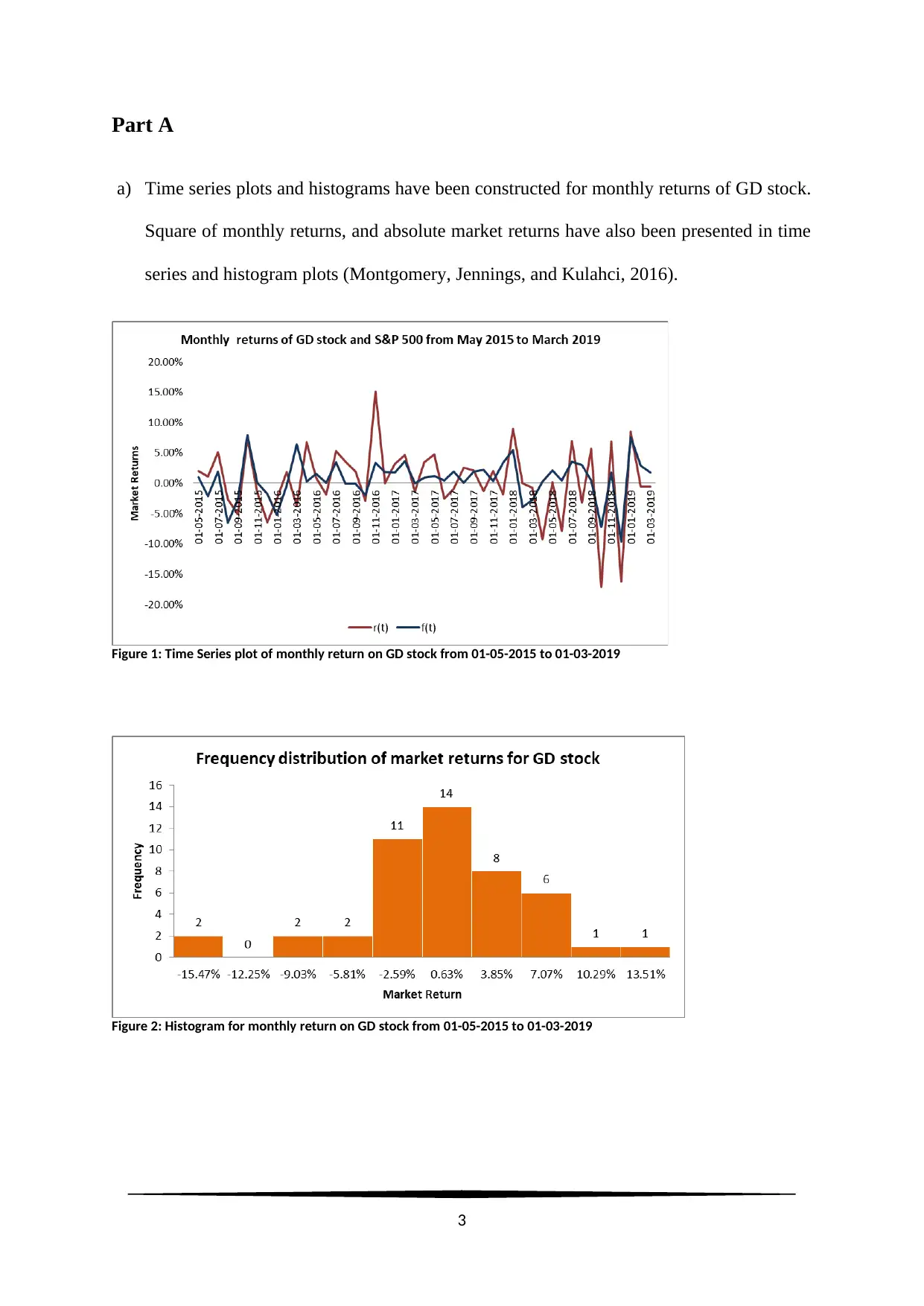
a) Time series plots and histograms have been constructed for monthly returns of GD stock.
Square of monthly returns, and absolute market returns have also been presented in time
series and histogram plots (Montgomery, Jennings, and Kulahci, 2016).
Figure 1: Time Series plot of monthly return on GD stock from 01-05-2015 to 01-03-2019
Figure 2: Histogram for monthly return on GD stock from 01-05-2015 to 01-03-2019
3

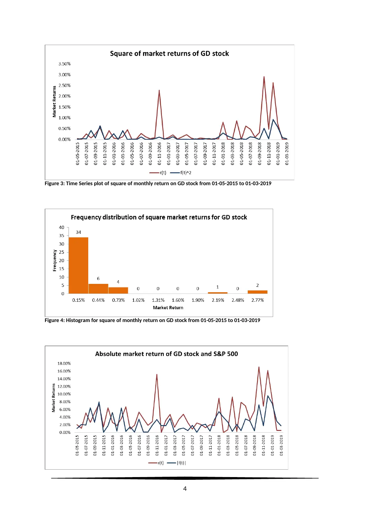
Figure 3: Time Series plot of square of monthly return on GD stock from 01-05-2015 to 01-03-2019
Figure 4: Histogram for square of monthly return on GD stock from 01-05-2015 to 01-03-2019
4

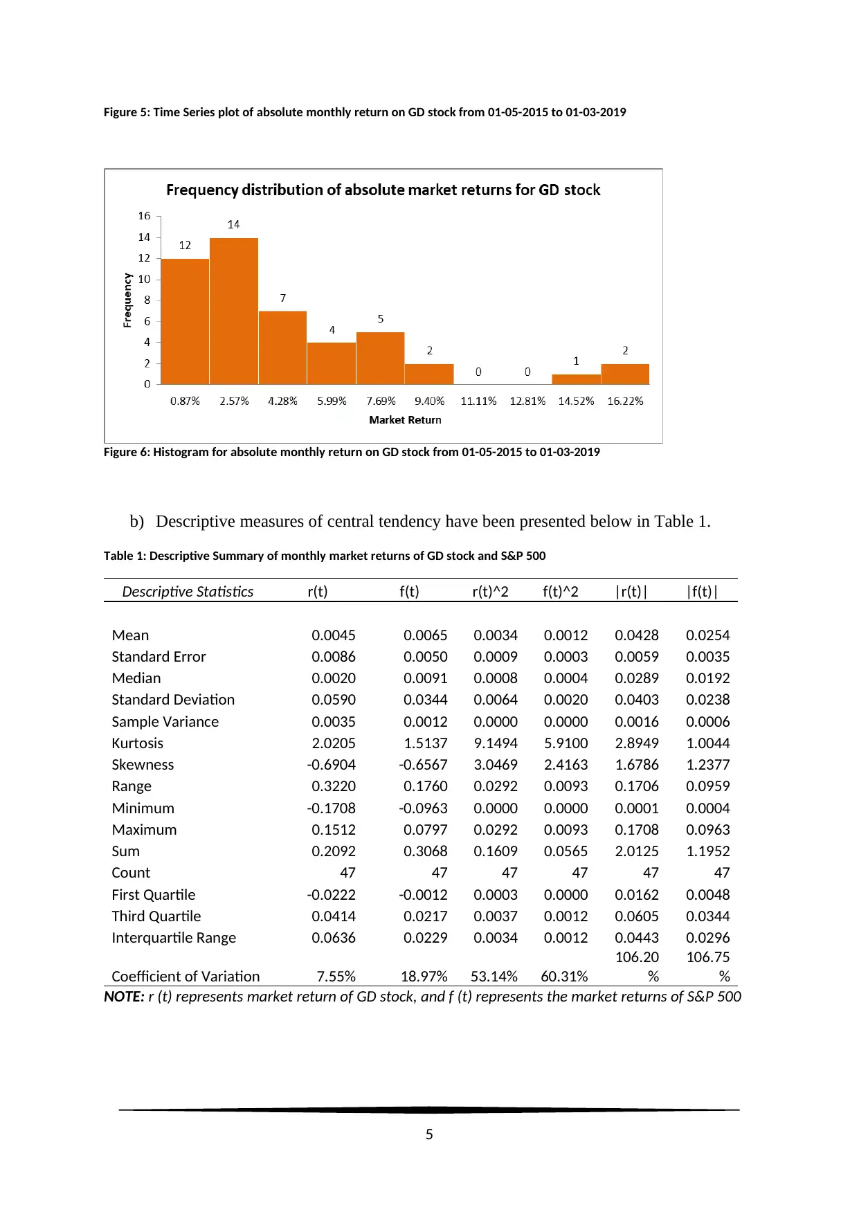
Figure 5: Time Series plot of absolute monthly return on GD stock from 01-05-2015 to 01-03-2019
Figure 6: Histogram for absolute monthly return on GD stock from 01-05-2015 to 01-03-2019
b) Descriptive measures of central tendency have been presented below in Table 1.
Table 1: Descriptive Summary of monthly market returns of GD stock and S&P 500
Descriptive Statistics r(t) f(t) r(t)^2 f(t)^2 |r(t)| |f(t)|
Mean 0.0045 0.0065 0.0034 0.0012 0.0428 0.0254
Standard Error 0.0086 0.0050 0.0009 0.0003 0.0059 0.0035
Median 0.0020 0.0091 0.0008 0.0004 0.0289 0.0192
Standard Deviation 0.0590 0.0344 0.0064 0.0020 0.0403 0.0238
Sample Variance 0.0035 0.0012 0.0000 0.0000 0.0016 0.0006
Kurtosis 2.0205 1.5137 9.1494 5.9100 2.8949 1.0044
Skewness -0.6904 -0.6567 3.0469 2.4163 1.6786 1.2377
Range 0.3220 0.1760 0.0292 0.0093 0.1706 0.0959
Minimum -0.1708 -0.0963 0.0000 0.0000 0.0001 0.0004
Maximum 0.1512 0.0797 0.0292 0.0093 0.1708 0.0963
Sum 0.2092 0.3068 0.1609 0.0565 2.0125 1.1952
Count 47 47 47 47 47 47
First Quartile -0.0222 -0.0012 0.0003 0.0000 0.0162 0.0048
Third Quartile 0.0414 0.0217 0.0037 0.0012 0.0605 0.0344
Interquartile Range 0.0636 0.0229 0.0034 0.0012 0.0443 0.0296
Coefficient of Variation 7.55% 18.97% 53.14% 60.31%
106.20
%
106.75
%
NOTE: r (t) represents market return of GD stock, and f (t) represents the market returns of S&P 500
5

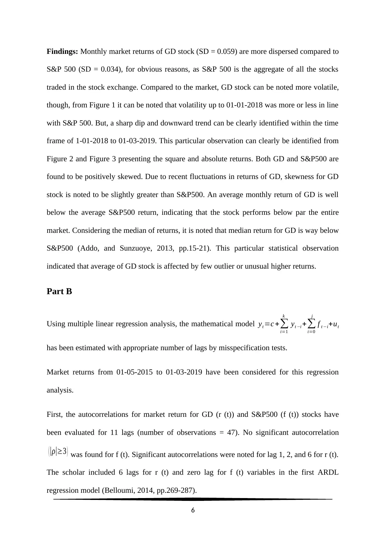
Findings: Monthly market returns of GD stock (SD = 0.059) are more dispersed compared to
S&P 500 (SD = 0.034), for obvious reasons, as S&P 500 is the aggregate of all the stocks
traded in the stock exchange. Compared to the market, GD stock can be noted more volatile,
though, from Figure 1 it can be noted that volatility up to 01-01-2018 was more or less in line
with S&P 500. But, a sharp dip and downward trend can be clearly identified within the time
frame of 1-01-2018 to 01-03-2019. This particular observation can clearly be identified from
Figure 2 and Figure 3 presenting the square and absolute returns. Both GD and S&P500 are
found to be positively skewed. Due to recent fluctuations in returns of GD, skewness for GD
stock is noted to be slightly greater than S&P500. An average monthly return of GD is well
below the average S&P500 return, indicating that the stock performs below par the entire
market. Considering the median of returns, it is noted that median return for GD is way below
S&P500 (Addo, and Sunzuoye, 2013, pp.15-21). This particular statistical observation
indicated that average of GD stock is affected by few outlier or unusual higher returns.
Part B
Using multiple linear regression analysis, the mathematical model yt =c +∑
i=1
k
yt −i +∑
i=0
j
f t −i+ut
has been estimated with appropriate number of lags by misspecification tests.
Market returns from 01-05-2015 to 01-03-2019 have been considered for this regression
analysis.
First, the autocorrelations for market return for GD (r (t)) and S&P500 (f (t)) stocks have
been evaluated for 11 lags (number of observations = 47). No significant autocorrelation
(|ρ|≥3 ) was found for f (t). Significant autocorrelations were noted for lag 1, 2, and 6 for r (t).
The scholar included 6 lags for r (t) and zero lag for f (t) variables in the first ARDL
regression model (Belloumi, 2014, pp.269-287).
6

Model: The ARDL model was framed as
Y t =c +∑
i =1
k
βi Y t −i+∑
i=0
j
ηi f t−i+ut
where ut
represents residuals of the model. Here, Y (t) is considered in place of r (t). k = number of
lags for Y (t), and j = number of lags for f (t).
Let ut (t =1, 2, 3… T) be the estimated residuals from the regression model, where,
ut=ρ1 ut−1+ ρ2 ut−2+ ρ3 ut −3+. .. .+ ρk ut−k +et Where ρi ' s denote the auto correlations at
ith
order.
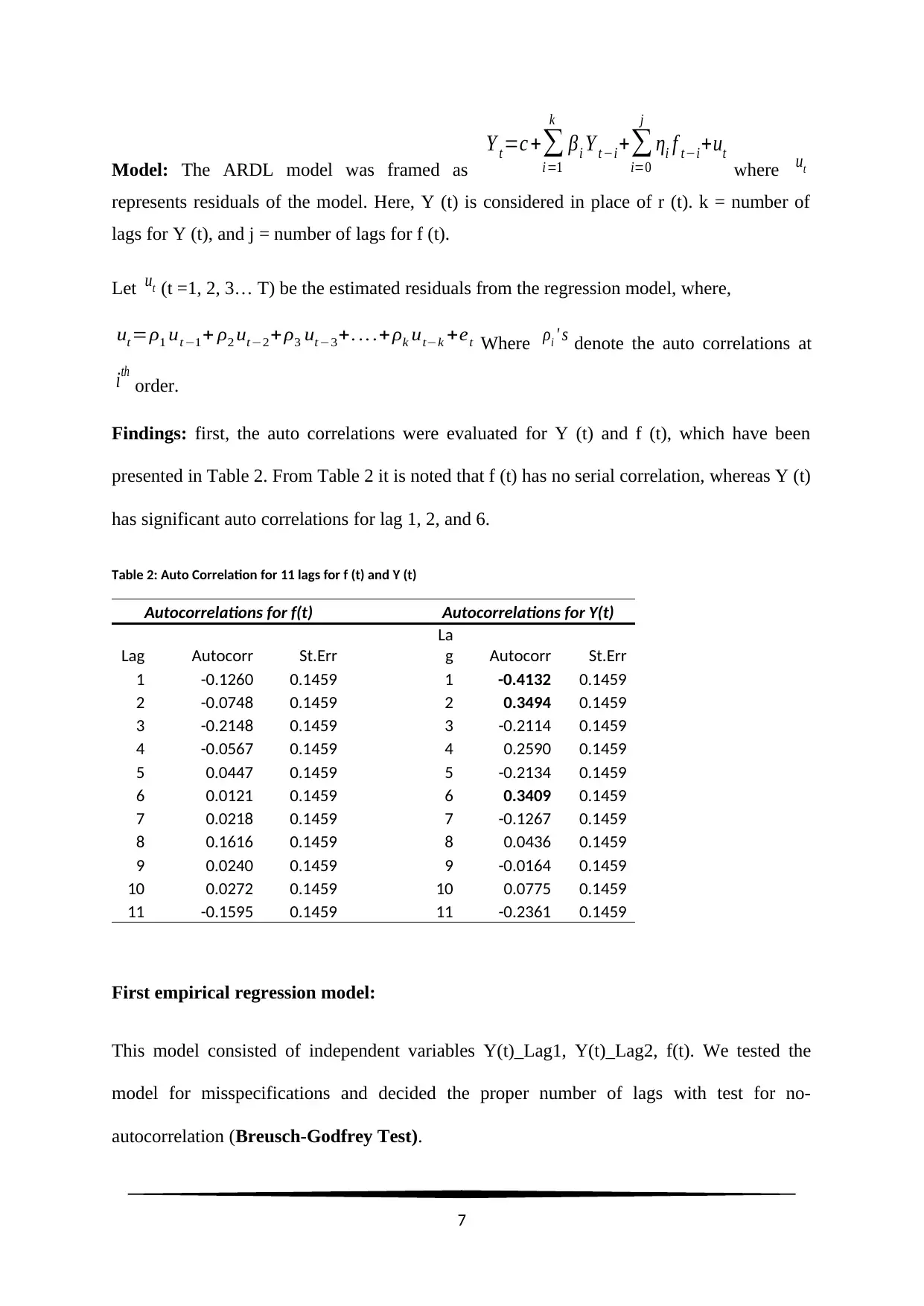
Findings: first, the auto correlations were evaluated for Y (t) and f (t), which have been
presented in Table 2. From Table 2 it is noted that f (t) has no serial correlation, whereas Y (t)
has significant auto correlations for lag 1, 2, and 6.
Table 2: Auto Correlation for 11 lags for f (t) and Y (t)
Autocorrelations for f(t) Autocorrelations for Y(t)
Lag Autocorr St.Err
La
g Autocorr St.Err
1 -0.1260 0.1459 1 -0.4132 0.1459
2 -0.0748 0.1459 2 0.3494 0.1459
3 -0.2148 0.1459 3 -0.2114 0.1459
4 -0.0567 0.1459 4 0.2590 0.1459
5 0.0447 0.1459 5 -0.2134 0.1459
6 0.0121 0.1459 6 0.3409 0.1459
7 0.0218 0.1459 7 -0.1267 0.1459
8 0.1616 0.1459 8 0.0436 0.1459
9 0.0240 0.1459 9 -0.0164 0.1459
10 0.0272 0.1459 10 0.0775 0.1459
11 -0.1595 0.1459 11 -0.2361 0.1459
First empirical regression model:
This model consisted of independent variables Y(t)_Lag1, Y(t)_Lag2, f(t). We tested the
model for misspecifications and decided the proper number of lags with test for no-
autocorrelation (Breusch-Godfrey Test).
7

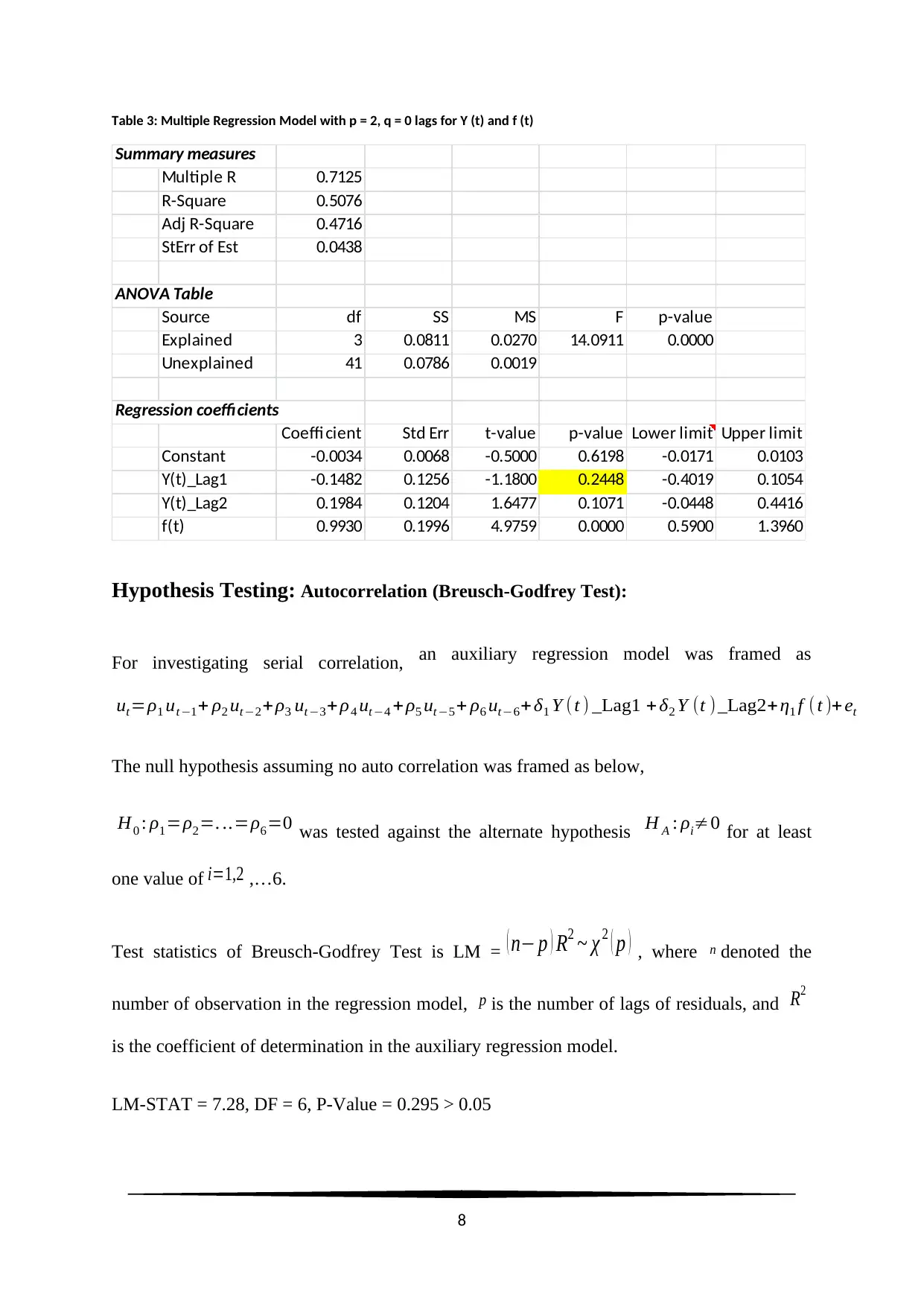
Table 3: Multiple Regression Model with p = 2, q = 0 lags for Y (t) and f (t)
Summary measures
Multiple R 0.7125
R-Square 0.5076
Adj R-Square 0.4716
StErr of Est 0.0438
ANOVA Table
Source df SS MS F p-value
Explained 3 0.0811 0.0270 14.0911 0.0000
Unexplained 41 0.0786 0.0019
Regression coefficients
Coeffi cient Std Err t-value p-value Lower limit Upper limit
Constant -0.0034 0.0068 -0.5000 0.6198 -0.0171 0.0103
Y(t)_Lag1 -0.1482 0.1256 -1.1800 0.2448 -0.4019 0.1054
Y(t)_Lag2 0.1984 0.1204 1.6477 0.1071 -0.0448 0.4416
f(t) 0.9930 0.1996 4.9759 0.0000 0.5900 1.3960
Hypothesis Testing: Autocorrelation (Breusch-Godfrey Test):
For investigating serial correlation, an auxiliary regression model was framed as
ut=ρ1 ut −1+ ρ2 ut −2+ ρ3 ut −3+ ρ4 ut −4 + ρ5 ut −5+ ρ6 ut−6+ δ1 Y (t ) _Lag1 + δ2 Y (t )_Lag2+ η1 f (t )+ et
The null hypothesis assuming no auto correlation was framed as below,
H0 : ρ1=ρ2=. ..=ρ6=0 was tested against the alternate hypothesis H A : ρi≠0 for at least
one value of i=1,2 ,…6.
Test statistics of Breusch-Godfrey Test is LM = ( n− p ) R2 ~ χ 2 ( p ) , where n denoted the
number of observation in the regression model, p is the number of lags of residuals, and R2
is the coefficient of determination in the auxiliary regression model.
LM-STAT = 7.28, DF = 6, P-Value = 0.295 > 0.05
8

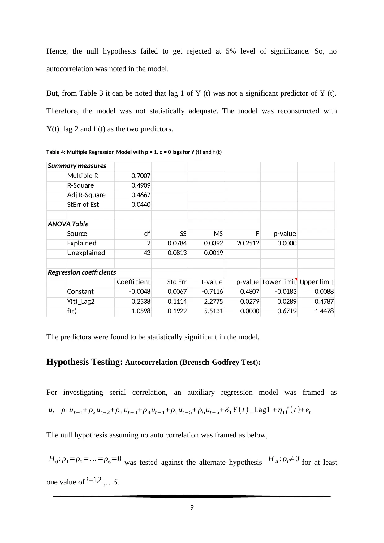
Hence, the null hypothesis failed to get rejected at 5% level of significance. So, no
autocorrelation was noted in the model.
But, from Table 3 it can be noted that lag 1 of Y (t) was not a significant predictor of Y (t).
Therefore, the model was not statistically adequate. The model was reconstructed with
Y(t)_lag 2 and f (t) as the two predictors.
Table 4: Multiple Regression Model with p = 1, q = 0 lags for Y (t) and f (t)
Summary measures
Multiple R 0.7007
R-Square 0.4909
Adj R-Square 0.4667
StErr of Est 0.0440
ANOVA Table
Source df SS MS F p-value
Explained 2 0.0784 0.0392 20.2512 0.0000
Unexplained 42 0.0813 0.0019
Regression coefficients
Coeffi cient Std Err t-value p-value Lower limit Upper limit
Constant -0.0048 0.0067 -0.7116 0.4807 -0.0183 0.0088
Y(t)_Lag2 0.2538 0.1114 2.2775 0.0279 0.0289 0.4787
f(t) 1.0598 0.1922 5.5131 0.0000 0.6719 1.4478
The predictors were found to be statistically significant in the model.
Hypothesis Testing: Autocorrelation (Breusch-Godfrey Test):
For investigating serial correlation, an auxiliary regression model was framed as
ut=ρ1 ut−1+ ρ2 ut−2+ρ3 ut−3+ ρ4 ut −4 + ρ5 ut−5+ ρ6 ut−6+ δ1 Y (t ) _Lag1 + η1 f (t )+ et
The null hypothesis assuming no auto correlation was framed as below,
H0 : ρ1=ρ2=. ..=ρ6=0 was tested against the alternate hypothesis H A : ρi≠0 for at least
one value of i=1,2 ,…6.
9

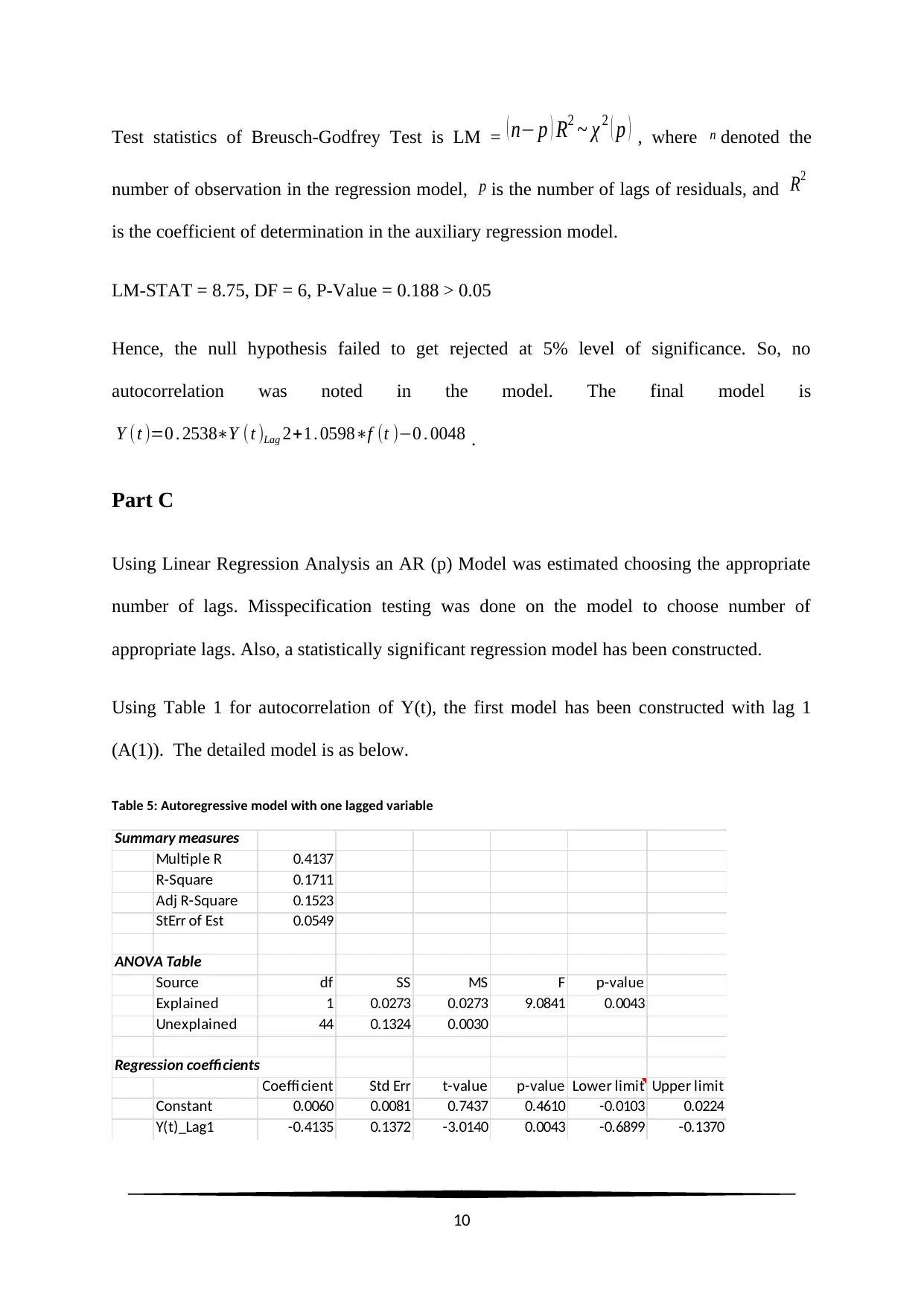
Test statistics of Breusch-Godfrey Test is LM = ( n− p ) R2 ~ χ 2 ( p ) , where n denoted the
number of observation in the regression model, p is the number of lags of residuals, and R2
is the coefficient of determination in the auxiliary regression model.
LM-STAT = 8.75, DF = 6, P-Value = 0.188 > 0.05
Hence, the null hypothesis failed to get rejected at 5% level of significance. So, no
autocorrelation was noted in the model. The final model is
Y ( t )=0 . 2538∗Y ( t )Lag 2+1. 0598∗f (t )−0 . 0048 .
Part C
Using Linear Regression Analysis an AR (p) Model was estimated choosing the appropriate
number of lags. Misspecification testing was done on the model to choose number of
appropriate lags. Also, a statistically significant regression model has been constructed.
Using Table 1 for autocorrelation of Y(t), the first model has been constructed with lag 1
(A(1)). The detailed model is as below.
Table 5: Autoregressive model with one lagged variable
Summary measures
Multiple R 0.4137
R-Square 0.1711
Adj R-Square 0.1523
StErr of Est 0.0549
ANOVA Table
Source df SS MS F p-value
Explained 1 0.0273 0.0273 9.0841 0.0043
Unexplained 44 0.1324 0.0030
Regression coefficients
Coeffi cient Std Err t-value p-value Lower limit Upper limit
Constant 0.0060 0.0081 0.7437 0.4610 -0.0103 0.0224
Y(t)_Lag1 -0.4135 0.1372 -3.0140 0.0043 -0.6899 -0.1370
10

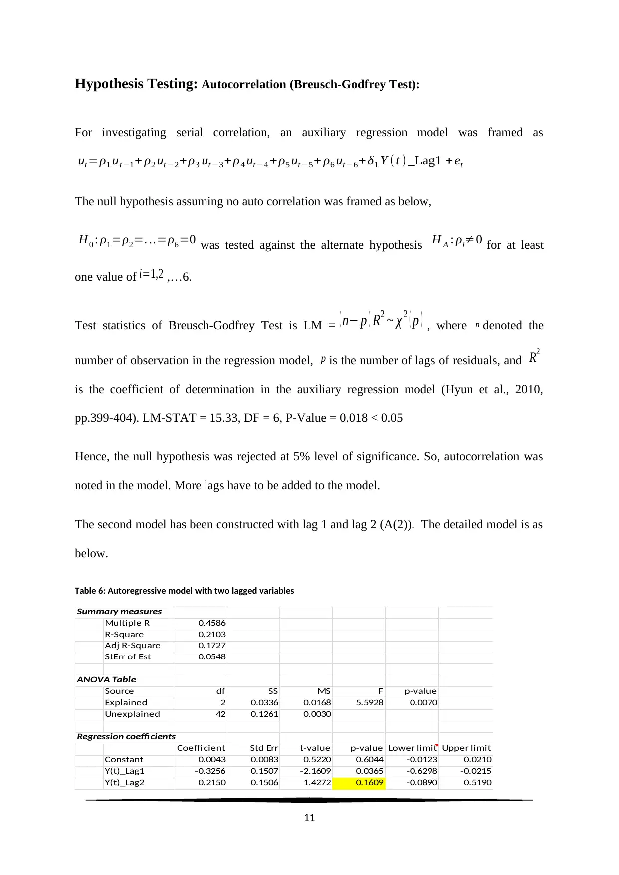
Hypothesis Testing: Autocorrelation (Breusch-Godfrey Test):
For investigating serial correlation, an auxiliary regression model was framed as
ut=ρ1 ut−1+ ρ2 ut−2+ρ3 ut −3+ρ4 ut −4 + ρ5 ut−5+ ρ6 ut−6+ δ1 Y (t ) _Lag1 + et
The null hypothesis assuming no auto correlation was framed as below,
H0 : ρ1=ρ2=. ..=ρ6=0 was tested against the alternate hypothesis H A : ρi≠0 for at least
one value of i=1,2 ,…6.
Test statistics of Breusch-Godfrey Test is LM = ( n− p ) R2 ~ χ 2 ( p ) , where n denoted the
number of observation in the regression model, p is the number of lags of residuals, and R2
is the coefficient of determination in the auxiliary regression model (Hyun et al., 2010,
pp.399-404). LM-STAT = 15.33, DF = 6, P-Value = 0.018 < 0.05
Hence, the null hypothesis was rejected at 5% level of significance. So, autocorrelation was
noted in the model. More lags have to be added to the model.
The second model has been constructed with lag 1 and lag 2 (A(2)). The detailed model is as
below.
Table 6: Autoregressive model with two lagged variables
Summary measures
Multiple R 0.4586
R-Square 0.2103
Adj R-Square 0.1727
StErr of Est 0.0548
ANOVA Table
Source df SS MS F p-value
Explained 2 0.0336 0.0168 5.5928 0.0070
Unexplained 42 0.1261 0.0030
Regression coefficients
Coeffi cient Std Err t-value p-value Lower limit Upper limit
Constant 0.0043 0.0083 0.5220 0.6044 -0.0123 0.0210
Y(t)_Lag1 -0.3256 0.1507 -2.1609 0.0365 -0.6298 -0.0215
Y(t)_Lag2 0.2150 0.1506 1.4272 0.1609 -0.0890 0.5190
11

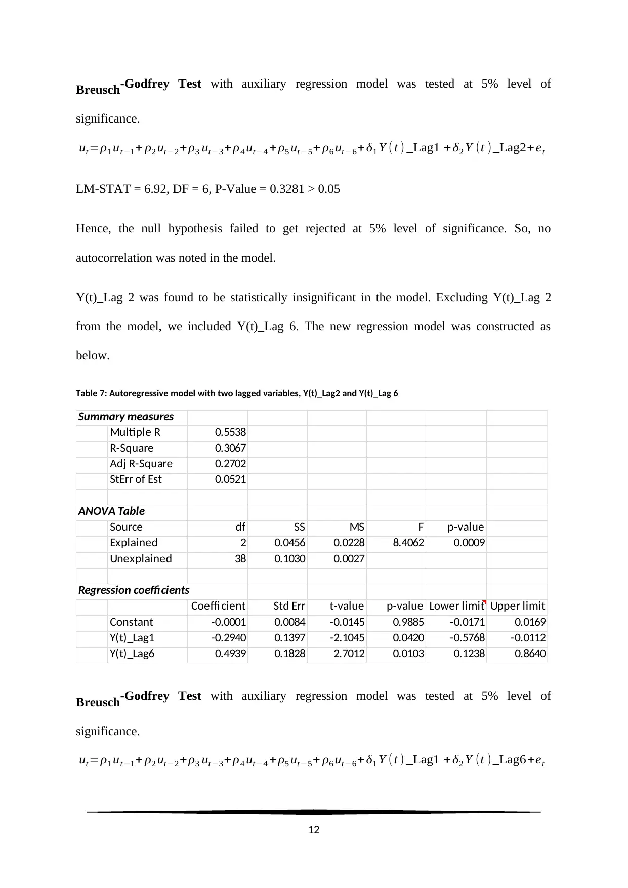
Breusch-Godfrey Test with auxiliary regression model was tested at 5% level of
significance.
ut=ρ1 ut −1+ ρ2 ut−2+ ρ3 ut −3+ ρ4 ut−4 + ρ5 ut−5+ ρ6 ut−6+ δ1 Y (t ) _Lag1 + δ2 Y (t )_Lag2+et
LM-STAT = 6.92, DF = 6, P-Value = 0.3281 > 0.05
Hence, the null hypothesis failed to get rejected at 5% level of significance. So, no
autocorrelation was noted in the model.
Y(t)_Lag 2 was found to be statistically insignificant in the model. Excluding Y(t)_Lag 2
from the model, we included Y(t)_Lag 6. The new regression model was constructed as
below.
Table 7: Autoregressive model with two lagged variables, Y(t)_Lag2 and Y(t)_Lag 6
Summary measures
Multiple R 0.5538
R-Square 0.3067
Adj R-Square 0.2702
StErr of Est 0.0521
ANOVA Table
Source df SS MS F p-value
Explained 2 0.0456 0.0228 8.4062 0.0009
Unexplained 38 0.1030 0.0027
Regression coefficients
Coeffi cient Std Err t-value p-value Lower limit Upper limit
Constant -0.0001 0.0084 -0.0145 0.9885 -0.0171 0.0169
Y(t)_Lag1 -0.2940 0.1397 -2.1045 0.0420 -0.5768 -0.0112
Y(t)_Lag6 0.4939 0.1828 2.7012 0.0103 0.1238 0.8640
Breusch-Godfrey Test with auxiliary regression model was tested at 5% level of
significance.
ut=ρ1 ut −1+ ρ2 ut−2+ ρ3 ut−3+ ρ4 ut−4 + ρ5 ut−5+ ρ6 ut−6+ δ1 Y ( t ) _Lag1 + δ2 Y (t ) _Lag6+et
12