SIT717 Assignment 1: Survey on ARIMA Models in Time Series Analysis

This report presents a survey on the application of Autoregressive Integrated Moving Average (ARIMA) models in time series data prediction. The survey explores the ARIMA model's components, including the AR, I, and MA terms, and their role in transforming non-stationary data into a stationary form, essential for reliable forecasting. It discusses the importance of stationarity, normality, and linearity tests in model validation. The report highlights ARIMA's prominence in business intelligence, emphasizing its ability to enhance the prediction of historical, current, and future trends, particularly in areas like economics, capacity planning, and weather forecasting. The survey also compares ARIMA with other machine learning techniques like LSTM and Prophet, underscoring ARIMA's effectiveness in time series analysis, and its ability to provide insights into the relationships between variables, supporting informed decision-making. The report also examines the tools used for modelling time series data using the ARIMA models and various tests that are essential for ensuring correct and reliable predictions about the projected values.

STATISTICS 1
A Brief Survey on Time Series Data Prediction Using ARIMA Models
Student’s name
Tutors name
Course
Institutional affiliation
City and state
Date

STATISTICS 2
Abstract
The survey explores the effect of ‘Auto-Regressive Integrated Moving
Averages’ (ARIMA), models in prediction of data based on time. ARIMA model
involves modelling of time series data in order to prediction. ARIMA models involves
many tests such as stationarity, normality and linearity. For the time series modelled
data, it is essential for the data to be stationary in order to provide reliable and
consistent results. The survey evaluated various other machine learning methods in
prediction. These techniques include; LSTM and PROPHET. The survey looked at
their differences and the behavior towards time series data. It was observed that
ARIMA is mostly used in prediction especially in business intelligence since it
enhances estimation of the historical, current and future forecasts.

STATISTICS 3
ARIMA models in prediction of time series data
1. Introduction
In the past years, time series data resolved by statisticians minus considering the
effects on their analysis that may be brought about by ‘non-stationeries’. Until
George. P and Jenkins. G came up with a monograph known as “Time series Analysis
forecast and control”. This tool helped in predicting so that the non-stationary data
could be transformed into stationary data. This would be done by ‘differencing’ series.
Time series data plays an essential role in future value forecast. Basing on past results,
time series is applied in forecasting changes in economics, capacity planning, weather
among others (Alsharif et al, 2019). However, features time-series data need specific
statistical methods to be applied. There are concepts that time series data uses and
these are autocorrelation, seasonality and stationary. In this paper, we are to discuss
the prominent time series method in forecasting and this method is known as ARIMA.
The ARIMA component is applied to transform time series data so as to ease the and
forecast future values in time series cheaply. ARIMA models give the best approach to
forecasting time series (Alsharif et al, 2019). The commonly used approaches in
forecasting time series data are ARIMA and exponential smoothing. These two
methods work hand in hand to solve problems. As exponential smoothing model relies
on describing data trends and seasonality, ARIMA models do describe the
autocorrelations within data. ARIMA is described as a group of models that
describes a specific time series relying on the previous values that is to say, its ‘own-
errors that are lagged on prediction errors. In this case, the ARIMA model is applied

STATISTICS 4
in prediction of values in future. The series that are not seasonal denies originality
and not a probability as the ‘white noise’ is transformed using ARIMA models. There
are three models that make an up model of ARIMA and these are presented by p, d
and q as discussed below;
P means the order of the ‘AR’ term
d means the number of ‘differencing’ needed to transform the time series data from
being non stationary to being stationary
q represents the order of the ‘MA’ term
If ‘seasonal pattern’ are observed in a time series, then there is a requirement of
summing up all seasonal terms so that the series become ‘Seasonal ARIMA ‘known as
“SARIMA”. For one to start forming an ARIMA model, the time series is made
stationary. The reason behind this is that the concept ‘Auto Regressive’ in ARIMA
shows it is a ‘linear regression model’ which applies its “lags” as forecasts. It is well
known that linear regression models perform well only if predictors are not correlated
and work separately. A time series is made stationary through finding the difference
between the past values and the current values (past values minus current values). In
cases when series are ‘large’, differencing can be made several times. Therefore, d
shows the highest times for differencing required to turn the series stationary.
However, in cases where time series are stationary, the d is zero (d = 0).
P represents the ‘Auto Regressive’ (AR) order of the term. This is the number of
“lags” of Y that are applied as predictors. On the other hand, q means ‘moving
Average’ order of the term. It is the “lagged” predicated errors that are meant to be

STATISTICS 5
fixed in the ARIMA model.
2. Objectives of the Survey
This paper intends to carry out a survey on the ARIMA models’ usage in
predicting the time series data. In time series data, prediction finds several
applications in different sectors of industries or businesses. The reason as to why
ARIMA models are use is that most of the machine languages do not give the clear
image of predictions especially in the businesses involving in sales and others dealing
in financial matters. ARIMA is considered as the best model to interpret and evaluate
the time series data to achieve the stipulated goals or objectives. It enhances the
prediction of demand of products through optimization of production and warehouse
storage to anticipate the level of funds (money) from sales and even for future stock
values of price.
3. Tools used to model time series data
There are many choices of software that are used in modelling of time series
prediction. Through prediction using such tools, the ARIMA models are produced to
explain the data about variables needed to be studied. ARIMA is the statistical
technique that helps in projecting the future figures about the series basing on its own
inertia. To use ARIMA models, the data in the question should be at least 30 and
above historical data points for reliability issues and consistence. The ARIMA models
using time series data can be modeled in tools such as Python, R-language, Matlab,
STATA, MINITAB and many other languages. Most significant is that, before
reaching to the ‘sophisticated time series data’ some other models that form the
fountain of further predictions (ICDM, 2018a). It is believed that if the complicated
methods do not provide and yield reliable results, therefore there is no need of using
such methods. However, several procedures while using the ARIMA models in order
to present the clear results about time series data (Lucey et al, 2018). Mean; this is
among the procedures followed when modelling data since it shows the forecasts that
are equivalent to the value of mean about time series data. Naïve; this procedure
shows the equivalence of the forecasts and the previous values about time series and

STATISTICS 6
lastly is the seasonal naïve. Seasonal naïve involves the forecasts for a specified
season that are equivalent to the values of seasonal period that is full. For instance,
when the predicted values of January 2019 are equivalent to those of time series
values in January of 2018.
The ARIMA models can forecast the Time Series Model (TSLM) as the
linear regression equations that forecasts the value needed about given variables. The
linear regression can be either linear trend or seasonality trends.
Yt = ao + a1X1t + a2X2t + ……. + anXnt + et
Where Xit are the explanatory variables, ai and b are the coefficients of
regression to be estimated. The most used trends in prediction time series data using
ARIMA models are linear trends and the seasonality effects. Also, the Seasonality
predictors are mostly in form of dummy variables which indicate the period of time
(monthly, quarterly, weekly and yearly) under which the predictions are made.
Furthermore, in ARIMA modelling other than linear trend and seasonality, there are
other several methods in prediction such as exponential smoothing and others. Most
significant in this paper is to assess the idea of prediction for future values about time
series as the ‘weighted average’ for last values whereby the weights that reduce the
time exponentially (Lucey et al, 2018). Besides, the method can as well be extended
to involved (method of Holt known as double exponential smoothing) or trend using
Holt Winter’s method. More so, the trends and seasonality coefficients in these
models can be determined by use of weighted averages of given expressions. In
addition, exponential smoothing is vital in predicting time series, the fundamental
point of view here is to forecast future outcomes whereby the attached weights
decrease exponentially as time changes. The equation of smoothing can be stated as
below;
Yt = a yt-1 + a(1-a) yt-2 + a(1-a)2 yt-3 + ……….
Where a (0,1) is smoothing parameter that are estimated. The displayed
method above can as well be extended to involve the doubled ‘exponential
smoothing’.

STATISTICS 7
The ‘Autoregressive Integrated Moving Average’ techniques completely use
various approaches. Autoregressive (AR) approach takes into account for the impact
of previous values about the predicted values.
Yt=a1yt-1+ a2yt-2+et; whereas the model of Moving Average (MA) that impacts
the noise of the estimated values of time series.
Yt=et+b1et-1+b2et-2.
Whereby et is the ‘random noise’ terms and each term about the random noise
have influence on three (3) yt values consecutively. In the current situation random
noise terms bring about the image of unexpected events such as statements made by
politicians that affect the stock markets (Sapankevych & Sankar, 2009) . The
combination of AR and MA models is read as ARMA and it can be shown in simple
way as:
Yt=et+b1et-1+b2et-2+a1yt-1+a2yt-2. As per the combination of AR and MA
(ARMA), the integrated portion for ARIMA is likely to correspond to technical
matters especially on how the ARMA models can be plotted and fitted out.
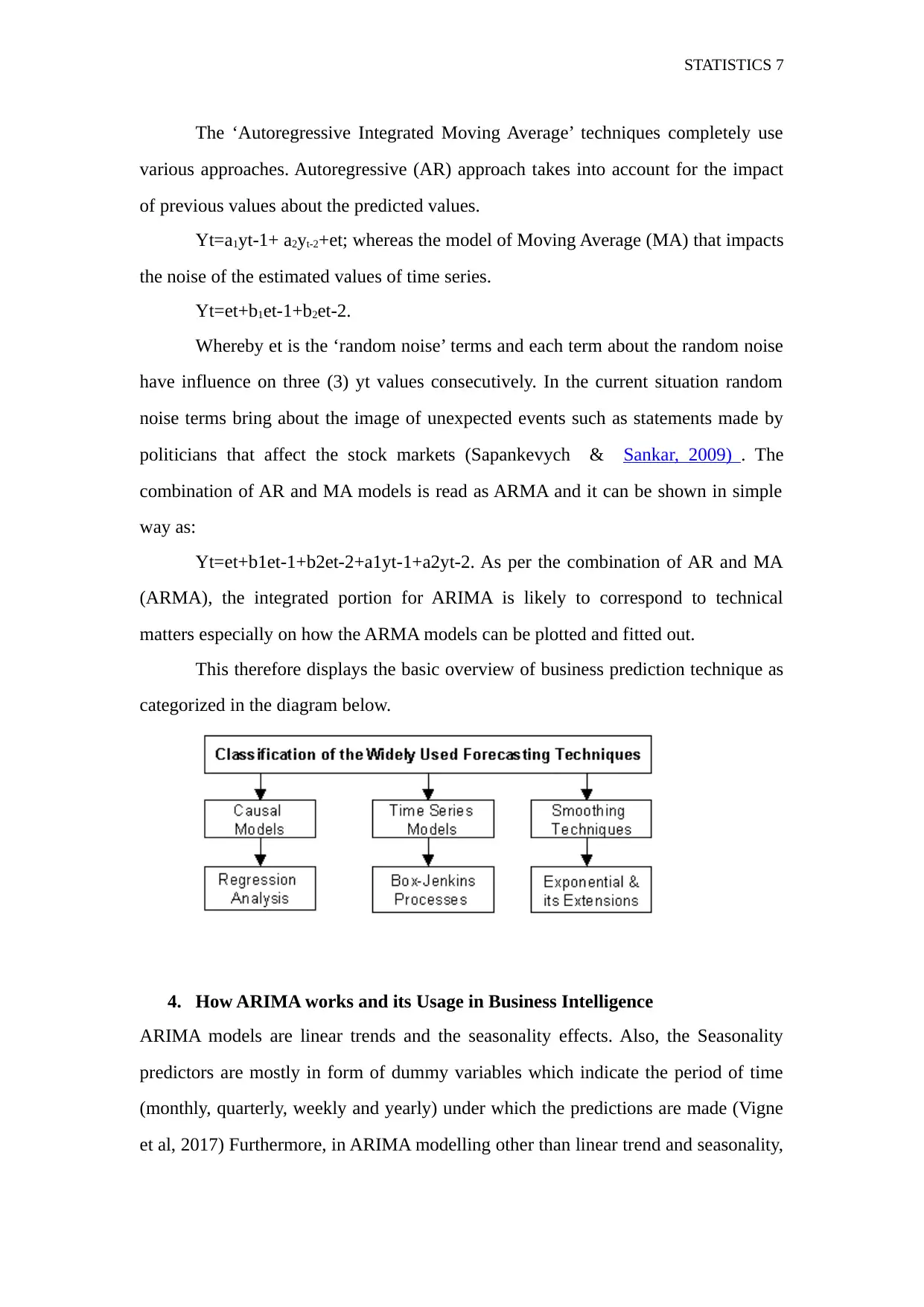
This therefore displays the basic overview of business prediction technique as
categorized in the diagram below.
4. How ARIMA works and its Usage in Business Intelligence
ARIMA models are linear trends and the seasonality effects. Also, the Seasonality
predictors are mostly in form of dummy variables which indicate the period of time
(monthly, quarterly, weekly and yearly) under which the predictions are made (Vigne
et al, 2017) Furthermore, in ARIMA modelling other than linear trend and seasonality,

STATISTICS 8
there are other several methods in prediction such as exponential smoothing and
others. Most significant in this paper is to assess the idea of prediction for future
values about time series as the average weighted values of previous items whereby
weights that reduce the time exponentially (Haider et al, 2019).
While using ARIMA technique in predicting the time series data, several tests should
be done to ensure correct, reliable, consistence predictions about the projected values.
These tests include; stationarity tests, linearity tests and normality tests. For
stationarity tests, STATA package, R-language, Python among others produce the tests
to ensure stationarity of the time series data. These methods of Stationarity tests
include; Augmented Dickey Fuller Test, Philp Perron tests among others. Also,
Normality tests are used to ensure data emanates from the normally distributed
population to ensure consistency of values. Normality can be tested using Shapiro
Wilkson’s Test and so on. Lastly, Linearity tests are also vital in modelling of time
series data using the technique of ARMA. The linearity tests are used to ensure the
relationships between the variables under the study. For example, by comparing the
relationship between sales and profitability levels in businesses, ARIMA models are
useful to predict and show the linear relationships (Sapankevych & Sankar, 2009) . The
relationships help to provide conclusions about the prices thus enhancing policy
making. Furthermore, most of the businesses around the globe succeed as time also
moves as time is left as dependent pattern. This helps to understanding the historical
values, analyzing the clear view of current and future values about the companies’
operations for better engagement with their customers (I CD M, 2 01 8 b ) .
5. Difference among several methods
There are other several techniques which are used in prediction of time series data.
These techniques (Machine learning models) include; LSTM and PROPHET. LSTM;
This refer s to the machine languages developed by the human being with the
recurrent neutral network architecture. This is fundamental technique used in the
fields of machine learning methods. On the other hand, networks that are neutral are
sometimes called standard feedforward. By considering Long short term memory, the

STATISTICS 9
connections of feedback which change the values into computers of general purpose
computes anything that machines perform (Haider et al, 2019). They are used in
predicting sequence problems especially in complex ones like machine translation and
recognition of the speech.
The other technique in time series is called PROPHET, this involves the
prediction of data based on time. It is further based on the additive model whereby it
involves the trends that are non-linear and plotted out. The data about Facebook
Prophet can be categorized in terms of monthly, monthly and so on (Taylor
&Letham,2017). It is hard for many machine learning methods to give high quality
predictions since it requires substantial requirement of experience and ‘specific
skills’. This method allows both the non-experts and the experts in the field of
forecast the quality.
Generally, ARIMA technique provides specific and well understandable
results that prevail in the day today businesses and other organizations compared to
others techniques of prediction about time series data. It provides simple and clear
models such as the linear trends which are used to compare prices, sales and
profitability of levels of the businesses. This is because ARIMA models behave to be
the best statistical models since they provide technical considerations for the
businessmen to predict their prices, sales and other variables in question. This
therefore shows that ARIMA models are vital as per data that depend on time is
concerned.
Related Studies
The study conducted by McNally in 2018 on the techniques of modelling time
series data using LSTM other than ARIMA methods. McNally focused on the opening

STATISTICS 10
and closing values of the cryptocurrencies using LSTM methods of prediction. He
found out that the accuracy level of the currency using open values was 52.8% with
its corresponding RSME of 5.5% (McNally, 2018).
Andrew (2018) conducted a study on the exploration on interconnections of
cryptocurrencies by the use of neutral networks such as ARIMA and PROPHET
models. The research investigated on the values that are zeroed on the time factor
about evaluation of prices. The models such as ARIMA and PROPHET identified
important features about the data sets of the prices forecasted.
6. Conclusions
In conclusion, selecting the model is regarded as a problem or a difficulty
while using machine learning methods for predictions. One of the ways how such a
problem can be evaluated is to separate several data into train and sets of tests for
computations of errors after understanding technique used to forecast time series data.
The basics of ARIMA models and time series prediction has been explained above.
While selecting machine learning model for forecasting, it is not easy to choose the
clear idea of which approach to use since all of them as discussed in this paper
provides forecasting of the time series data. Most significant is that, before reaching
to the ‘sophisticated time series data’ some other models that form the fountain of
further predictions. It is believed that if the complicated methods do not provide and
yield reliable results, therefore there is no need of using such methods. However,
several procedures while using the ARIMA models in order to present the clear results
about time series data. However, the degree defers in terms of preciseness, clarity,
consistency, unbiasedness and others. It is evident that, without metrics in business or
any other organization, management may become nebulous. Estimation and
Prediction of the data about the variables helps organizations to tell whether they are
incurring profits or losses and even forecasting future outcomes basing on the
historical phenomenon. With ARIMA models, each business can be in position to
measure the success and set targets from the policies made after estimations of the

STATISTICS 11
data.
List of References
Alsharif, A.M., Younes, K.M. & Kim, J. 2019. Time Series ARIMA Model for
Prediction of Daily and Monthly Average Global Solar Radiation: The Case Study of
Seoul, South Korea. Retrieved from: https://www.mdpi.com/2073-8994/11/2/240
Haider , S. A., Naqvi S.R , Akram, T. Umar, A.G. , Shahzad, A. , Sial, M.R.,
ICDM. 2018a. 20th International Conference on Data Mining. Retrieved from:
http://www.wikicfp.com/cfp/servlet/event.showcfp?eventid=66339
ICDM. 2018 b. The 2018 IEEE International Conference on Data
Mining. Retrieved from:
http://www2.kansai-u.ac.jp/dslab/workshop/2018/DMS2018/
Khaliq, S. & Kamran, M. 2019. LSTM Neural Network Based Forecasting Model for
Wheat Production in Pakistan. Retrieved from: https://www.mdpi.com/2073-
4395/9/2/72
Lucey, B. M., Vigne, S. A., Ballester, L., Barbopoulos, L., Brzeszczynski, J.,
Carchano, O., Zaghini, A. 2018. Future directions in international financial
integration research - A crowdsourced perspective. International Review of Financial
Analysis, 55, 35–49.
MacNally, S. 2018. Predicting the Price of Bitcoin Using Machine Learning.
Retrieved from:
https://www.researchgate.net/publication/325633087_Predicting_the_Price_of_Bitcoi
n_Using _Machine_Learning
Sapankevych, I.N. & Sankar, R. 2009. Time Series Prediction Using Support Vector
Machines: A Survey. Publisher: IEEE. Retrieved from:
https://ieeexplore.ieee.org/document/4840324/references#references
Taylor S. &, Letham, B. 2017. Forecasting at scale. Retrieved from:
https://peerj.com/preprints/3190/
Vigne, S. A., Lucey, B. M., O’Connor, F. A., &Yarovaya, L. 2017. The financial

STATISTICS 12
economics of white precious metals-A survey. International Review of Financial
Analysis, 52, 292—30 8.