Time Series Analysis and Cointegration Assignment, ECN2005

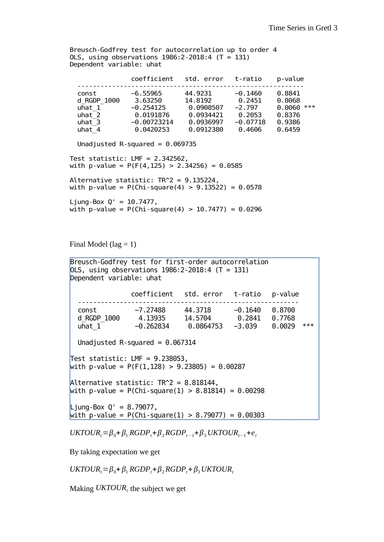
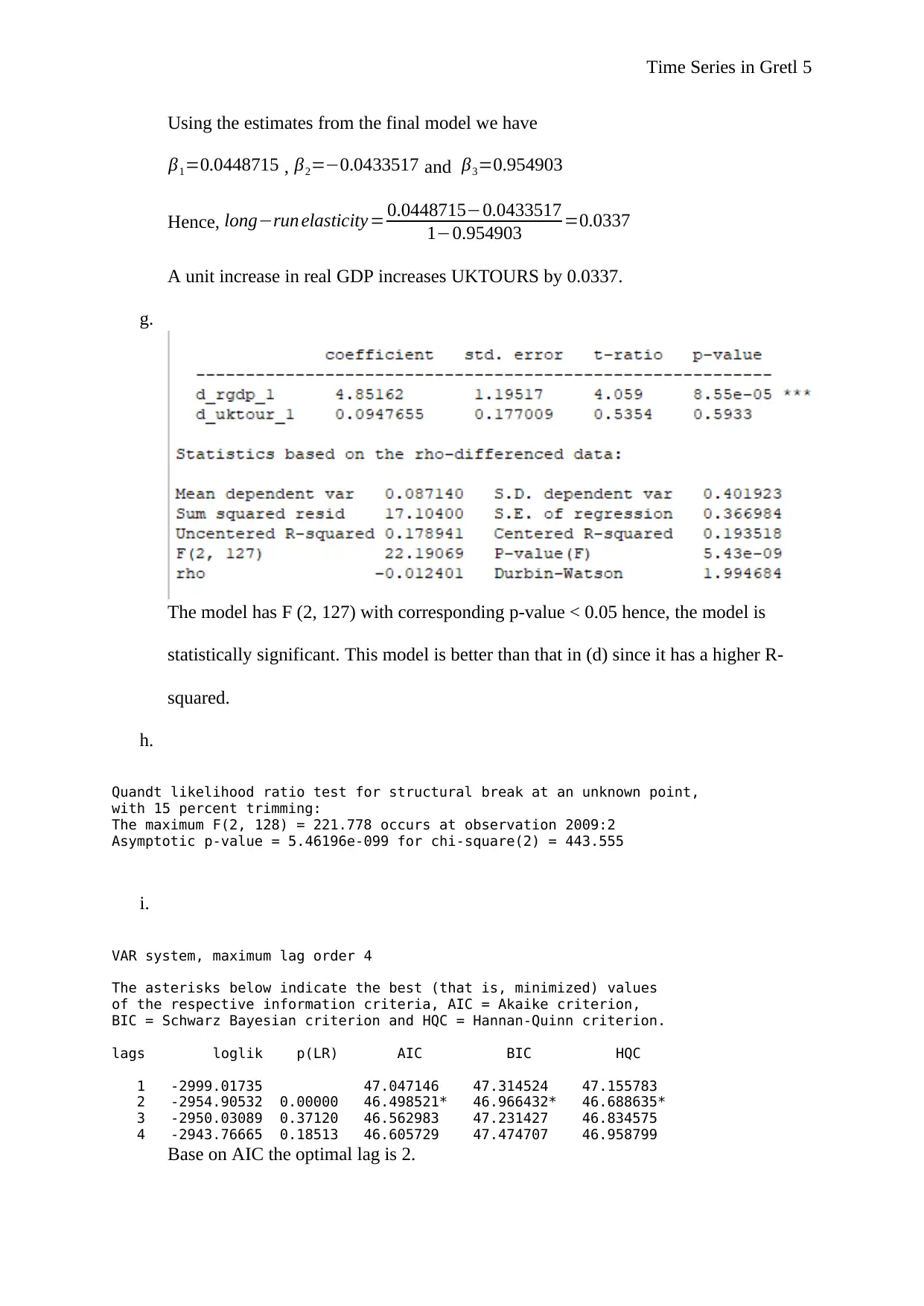
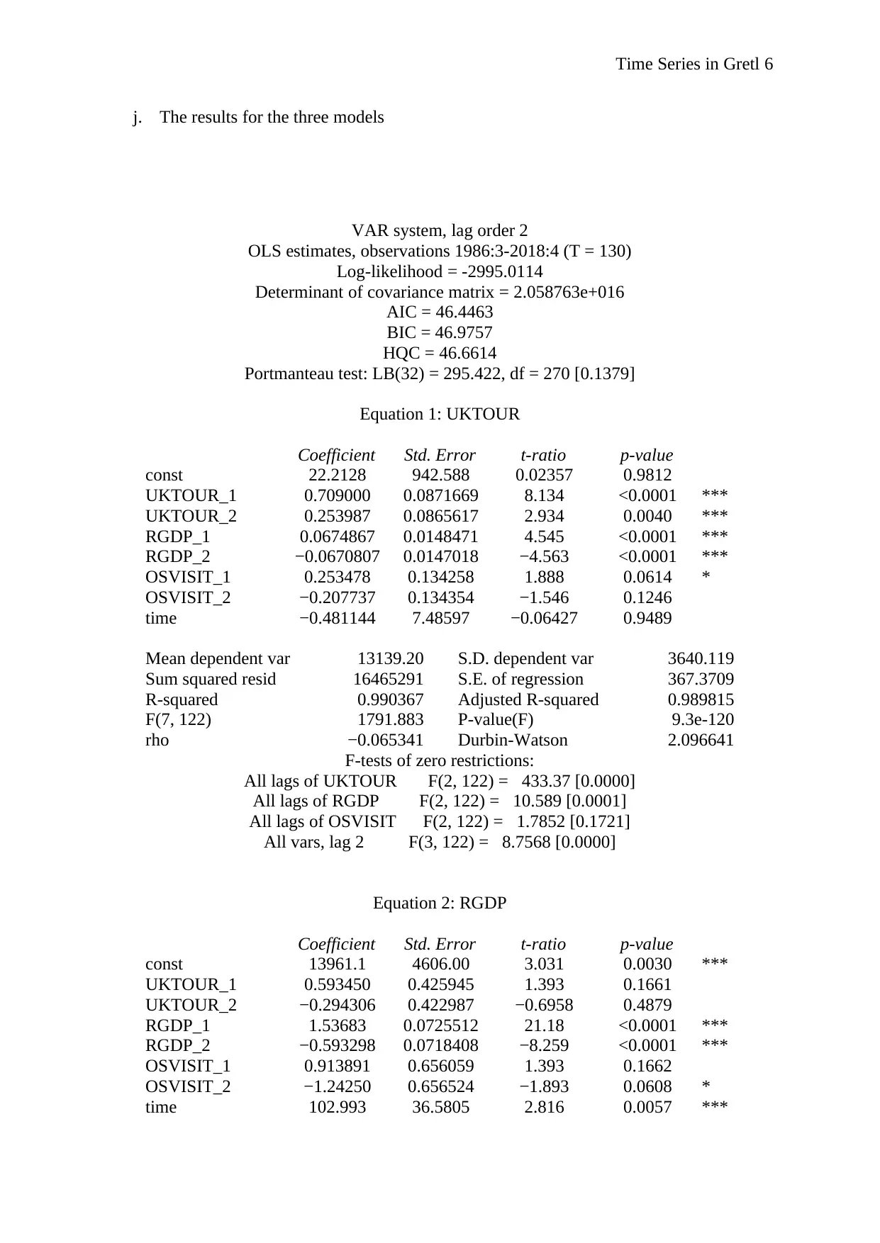
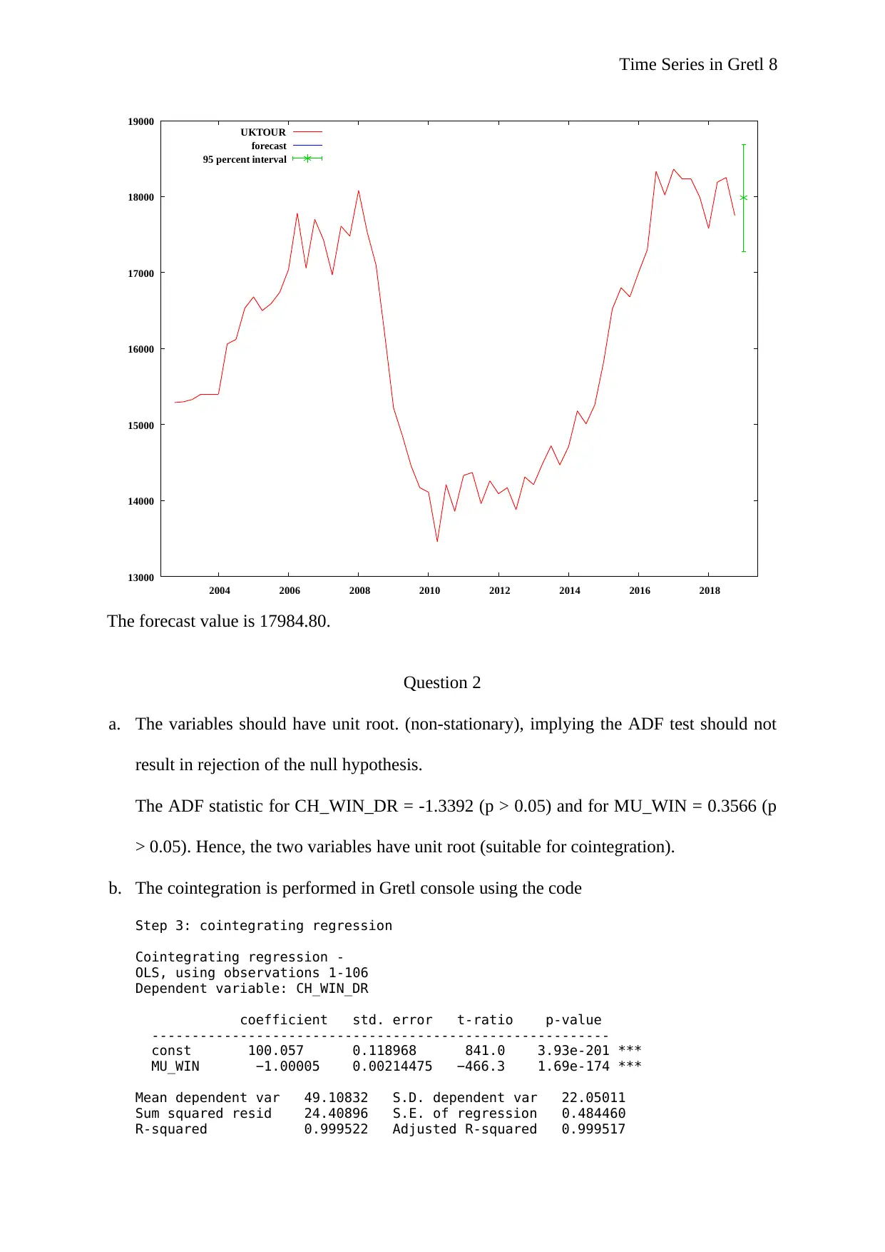
This document presents a comprehensive solution to a time series econometrics assignment for the ECN2005 course. The assignment utilizes the Gretl software to analyze quarterly data on UK real GDP, outbound tourist visits, and inbound tourist visits. The solution includes the application of Augmented Dickey-Fuller (ADF) tests to assess unit roots, transformations to achieve stationarity, and the development of Vector Autoregression (VAR) and Autoregressive Distributed Lag (ARDL) models. The analysis covers model specification, estimation, interpretation of coefficients, and the calculation of long-run elasticities. Furthermore, the solution investigates cointegration between variables and employs error correction models (ECM). The document provides detailed Gretl output, interpretations, and statistical tests, including the Quandt likelihood ratio test and portmanteau tests, to evaluate model validity and significance. The assignment covers topics like time series analysis, unit root testing, cointegration, VAR modeling, ARDL modeling, and error correction models.

Time Series in Gretl 1
Time Series Econometrics in Gretl
by[Name]
Course
Professor’s Name
Institution
Location of Institution
Date

Time Series in Gretl 2
Time Series Econometrics in Gretl
Question 1
a. The transformation made at this stage is on variable RGDP which is divided by 1000
to make it have the same units as UKTOURS and OSVISIT. The new variable is
named RGDP_1000.
b. In order to decide the model to use with ADF we plotted the trend of each variable as
shown in the figure 1 (see appendix). The results show that for UKTOUR,
RGDP_100, and OSVISIT the ADF statistic = -1.682 (p > 0.05), -2.071 (p > 0.05),
and -2.250 (p > 0.05) respectively. Therefore, unit root exists in all the variables.
c. Based on figure 1 have trend therefore, the best transformation to make the series
stationary is differencing. The figure 2 (see appendix) shows that the trend is removed
by first difference. On the differenced variables, for UKTOUR, RGDP_100, and
OSVISIT the ADF statistic = -3.505 (p < 0.05), -2.071 (p < 0.05), and -2.250 (p <
0.05) respectively. Therefore, all variables are stationary.
d. Taking into account the differenced variable the model of UKTOUR as a function of
RGDP is given as:
dUKTOURt=β0 + β1 dRGDPt +et
First Model (lag = 4)

Time Series in Gretl 3
Breusch-Godfrey test for autocorrelation up to order 4
OLS, using observations 1986:2-2018:4 (T = 131)
Dependent variable: uhat
coefficient std. error t-ratio p-value
-----------------------------------------------------------
const −6.55965 44.9231 −0.1460 0.8841
d_RGDP_1000 3.63250 14.8192 0.2451 0.8068
uhat_1 −0.254125 0.0908507 −2.797 0.0060 ***
uhat_2 0.0191876 0.0934421 0.2053 0.8376
uhat_3 −0.00723214 0.0936997 −0.07718 0.9386
uhat_4 0.0420253 0.0912380 0.4606 0.6459
Unadjusted R-squared = 0.069735
Test statistic: LMF = 2.342562,
with p-value = P(F(4,125) > 2.34256) = 0.0585
Alternative statistic: TR^2 = 9.135224,
with p-value = P(Chi-square(4) > 9.13522) = 0.0578
Ljung-Box Q' = 10.7477,
with p-value = P(Chi-square(4) > 10.7477) = 0.0296
Final Model (lag = 1)
Breusch-Godfrey test for first-order autocorrelation
OLS, using observations 1986:2-2018:4 (T = 131)
Dependent variable: uhat
coefficient std. error t-ratio p-value
----------------------------------------------------------
const −7.27488 44.3718 −0.1640 0.8700
d_RGDP_1000 4.13935 14.5704 0.2841 0.7768
uhat_1 −0.262834 0.0864753 −3.039 0.0029 ***
Unadjusted R-squared = 0.067314
Test statistic: LMF = 9.238053,
with p-value = P(F(1,128) > 9.23805) = 0.00287
Alternative statistic: TR^2 = 8.818144,
with p-value = P(Chi-square(1) > 8.81814) = 0.00298
Ljung-Box Q' = 8.79077,
with p-value = P(Chi-square(1) > 8.79077) = 0.00303
UKTOURt =β0+ β1 RGDPt + β2 RGDPt −1+ β3 UKTOURt−1 +et
By taking expectation we get
UKTOURt =β0+ β1 RGDPt + β2 RGDPt + β3 UKTOURt
Making UKTOURt the subject we get

Time Series in Gretl 4
UKTOURt = β0
1−β3
+ β1 + β2
1−β3
RGDPt
Therefore, the long-run elasticity is given by the formula
long−run elasticity= β1+ β2
1−β3
Hence, long−run elasticity=0.4464
A unit increase in GDP increase UKTOURS by 0.4464 units.
e. The estimates of the model are shown below
The model has F (2, 126) with corresponding p-value < 0.05 hence, the model is
statistically significant.
f. The ARDL is not a base model in Gretl, therefore, the script (appendix) was used to
import ADMBP package.
Model 1: OLS, using observations 1986:2-2018:4 (T = 131)
Dependent variable: UKTOUR
coefficient std. error t-ratio p-value
---------------------------------------------------------
UKTOUR_1 0.954903 0.0220707 43.27 2.87e-078 ***
RGDP 0.0448715 0.0144984 3.095 0.0024 ***
RGDP_1 −0.0433517 0.0146483 −2.960 0.0037 ***
The long-run elasticity is given by the formula
long−run elasticity= β1+ β2
1−β3

Time Series in Gretl 5
Using the estimates from the final model we have
β1=0.0448715 , β2=−0.0433517 and β3=0.954903
Hence, long−run elasticity= 0.0448715−0.0433517
1−0.954903 =0.0337
A unit increase in real GDP increases UKTOURS by 0.0337.
g.
The model has F (2, 127) with corresponding p-value < 0.05 hence, the model is
statistically significant. This model is better than that in (d) since it has a higher R-
squared.
h.
Quandt likelihood ratio test for structural break at an unknown point,
with 15 percent trimming:
The maximum F(2, 128) = 221.778 occurs at observation 2009:2
Asymptotic p-value = 5.46196e-099 for chi-square(2) = 443.555
i.
VAR system, maximum lag order 4
The asterisks below indicate the best (that is, minimized) values
of the respective information criteria, AIC = Akaike criterion,
BIC = Schwarz Bayesian criterion and HQC = Hannan-Quinn criterion.
lags loglik p(LR) AIC BIC HQC
1 -2999.01735 47.047146 47.314524 47.155783
2 -2954.90532 0.00000 46.498521* 46.966432* 46.688635*
3 -2950.03089 0.37120 46.562983 47.231427 46.834575
4 -2943.76665 0.18513 46.605729 47.474707 46.958799
Base on AIC the optimal lag is 2.

Time Series in Gretl 6
j. The results for the three models
VAR system, lag order 2
OLS estimates, observations 1986:3-2018:4 (T = 130)
Log-likelihood = -2995.0114
Determinant of covariance matrix = 2.058763e+016
AIC = 46.4463
BIC = 46.9757
HQC = 46.6614
Portmanteau test: LB(32) = 295.422, df = 270 [0.1379]
Equation 1: UKTOUR
Coefficient Std. Error t-ratio p-value
const 22.2128 942.588 0.02357 0.9812
UKTOUR_1 0.709000 0.0871669 8.134 <0.0001 ***
UKTOUR_2 0.253987 0.0865617 2.934 0.0040 ***
RGDP_1 0.0674867 0.0148471 4.545 <0.0001 ***
RGDP_2 −0.0670807 0.0147018 −4.563 <0.0001 ***
OSVISIT_1 0.253478 0.134258 1.888 0.0614 *
OSVISIT_2 −0.207737 0.134354 −1.546 0.1246
time −0.481144 7.48597 −0.06427 0.9489
Mean dependent var 13139.20 S.D. dependent var 3640.119
Sum squared resid 16465291 S.E. of regression 367.3709
R-squared 0.990367 Adjusted R-squared 0.989815
F(7, 122) 1791.883 P-value(F) 9.3e-120
rho −0.065341 Durbin-Watson 2.096641
F-tests of zero restrictions:
All lags of UKTOUR F(2, 122) = 433.37 [0.0000]
All lags of RGDP F(2, 122) = 10.589 [0.0001]
All lags of OSVISIT F(2, 122) = 1.7852 [0.1721]
All vars, lag 2 F(3, 122) = 8.7568 [0.0000]
Equation 2: RGDP
Coefficient Std. Error t-ratio p-value
const 13961.1 4606.00 3.031 0.0030 ***
UKTOUR_1 0.593450 0.425945 1.393 0.1661
UKTOUR_2 −0.294306 0.422987 −0.6958 0.4879
RGDP_1 1.53683 0.0725512 21.18 <0.0001 ***
RGDP_2 −0.593298 0.0718408 −8.259 <0.0001 ***
OSVISIT_1 0.913891 0.656059 1.393 0.1662
OSVISIT_2 −1.24250 0.656524 −1.893 0.0608 *
time 102.993 36.5805 2.816 0.0057 ***

Time Series in Gretl 7
Mean dependent var 389823.2 S.D. dependent var 77560.08
Sum squared resid 3.93e+08 S.E. of regression 1795.175
R-squared 0.999493 Adjusted R-squared 0.999464
F(7, 122) 34382.29 P-value(F) 9.1e-198
rho −0.120846 Durbin-Watson 2.236494
F-tests of zero restrictions:
All lags of UKTOUR F(2, 122) = 2.2727 [0.1074]
All lags of RGDP F(2, 122) = 1128 [0.0000]
All lags of OSVISIT F(2, 122) = 1.8581 [0.1604]
All vars, lag 2 F(3, 122) = 27.877 [0.0000]
Equation 3: OSVISIT
Coefficient Std. Error t-ratio p-value
const 344.677 630.896 0.5463 0.5858
UKTOUR_1 0.102436 0.0583428 1.756 0.0816 *
UKTOUR_2 −0.105551 0.0579377 −1.822 0.0709 *
RGDP_1 0.0152585 0.00993753 1.535 0.1273
RGDP_2 −0.0143105 0.00984022 −1.454 0.1484
OSVISIT_1 0.790214 0.0898621 8.794 <0.0001 ***
OSVISIT_2 0.0596767 0.0899259 0.6636 0.5082
time 4.94916 5.01053 0.9878 0.3252
Mean dependent var 6671.746 S.D. dependent var 1729.642
Sum squared resid 7376332 S.E. of regression 245.8897
R-squared 0.980887 Adjusted R-squared 0.979790
F(7, 122) 894.4213 P-value(F) 1.3e-101
rho −0.011195 Durbin-Watson 2.018986
F-tests of zero restrictions:
All lags of UKTOUR F(2, 122) = 1.6743 [0.1917]
All lags of RGDP F(2, 122) = 1.1808 [0.3105]
All lags of OSVISIT F(2, 122) = 149.51 [0.0000]
All vars, lag 2 F(3, 122) = 2.4175 [0.0696]
For the system as a whole
Null hypothesis: the longest lag is 1
Alternative hypothesis: the longest lag is 2
Likelihood ratio test: Chi-square(9) = 92.1626 [0.0000]
k. The figure below shows the forecast plot

Time Series in Gretl 8
13000
14000
15000
16000
17000
18000
19000
2004 2006 2008 2010 2012 2014 2016 2018
UKTOUR
forecast
95 percent interval
The forecast value is 17984.80.
Question 2
a. The variables should have unit root. (non-stationary), implying the ADF test should not
result in rejection of the null hypothesis.
The ADF statistic for CH_WIN_DR = -1.3392 (p > 0.05) and for MU_WIN = 0.3566 (p
> 0.05). Hence, the two variables have unit root (suitable for cointegration).
b. The cointegration is performed in Gretl console using the code
Step 3: cointegrating regression
Cointegrating regression -
OLS, using observations 1-106
Dependent variable: CH_WIN_DR
coefficient std. error t-ratio p-value
---------------------------------------------------------
const 100.057 0.118968 841.0 3.93e-201 ***
MU_WIN −1.00005 0.00214475 −466.3 1.69e-174 ***
Mean dependent var 49.10832 S.D. dependent var 22.05011
Sum squared resid 24.40896 S.E. of regression 0.484460
R-squared 0.999522 Adjusted R-squared 0.999517

Time Series in Gretl 9
Log-likelihood −72.57757 Akaike criterion 149.1551
Schwarz criterion 154.4820 Hannan-Quinn 151.3141
rho −0.114745 Durbin-Watson 2.228374
Step 4: testing for a unit root in uhat
Augmented Dickey-Fuller test for uhat
including 2 lags of (1-L)uhat
sample size 103
unit-root null hypothesis: a = 1
test without constant
model: (1-L)y = (a-1)*y(-1) + ... + e
estimated value of (a - 1): -1.0523
test statistic: tau_c(2) = -5.66814
asymptotic p-value 6.166e-006
1st-order autocorrelation coeff. for e: -0.013
lagged differences: F(2, 100) = 0.211 [0.8105]
There is evidence for a cointegrating relationship if:
(a) The unit-root hypothesis is not rejected for the individual variables, and
(b) the unit-root hypothesis is rejected for the residuals (uhat) from the
cointegrating regression.
There exist cointegration between the two probabilities.
c. The results are:
long-run matrix (alpha * beta')
CH_WIN_DR MU_WIN
CH_WIN_DR -0.028020 0.014362
MU_WIN 0.027429 -0.013846
d. Equation 2: d_MU_WIN
coefficient std. error t-ratio p-value
-------------------------------------------------------
EC1 0.0274768 0.0176605 1.556 0.1228
Mean dependent var 0.656365 S.D. dependent var 7.354476
Sum squared resid 5541.442 S.E. of regression 7.299527
R-squared 0.022746 Adjusted R-squared 0.022746
rho −0.008618 Durbin-Watson 2.016962
e. The hypothesis are:
H0 : EC 1=−1 against H0 : EC 1≠−1
Test statistic
t= EC 1+1
std . error
t= 0.0274+1
0.0176 =58.375
Decision

Time Series in Gretl 10
t >t105 ,0.025=2.274
Hence EC is different from -1.
f. The p-value for EC is 0.1228 which is greater than 0.05. Hence, the error correction term is
not significant in the ECM model. This result supported the results in (e).

Time Series in Gretl 11
Appendix
1. Figure 1
2000
4000
6000
8000
10000
12000
14000
16000
18000
20000
1990 1995 2000 2005 2010 2015
250
300
350
400
450
500
550
Value in Thousands
Year
Figure 1: Time Plot of Variables
UKTOUR (left)
OSVISIT (left)
RGDP_1000 (right)
2. ADF for UKTOUR
Augmented Dickey-Fuller test for uktour
testing down from 4 lags, criterion AIC
sample size 129
unit-root null hypothesis: a = 1
with constant and trend
including 2 lags of (1-L)uktour
model: (1-L)y = b0 + b1*t + (a-1)*y(-1) + ... + e
estimated value of (a - 1): -0.0298181
test statistic: tau_ct(1) = -1.3861
asymptotic p-value 0.8653
1st-order autocorrelation coeff. for e: -0.012
lagged differences: F(2, 124) = 2.710 [0.0705]
3. ADF for RGDP

Time Series in Gretl 12
Augmented Dickey-Fuller test for rgdp
testing down from 4 lags, criterion AIC
sample size 128
unit-root null hypothesis: a = 1
with constant and trend
including 3 lags of (1-L)rgdp
model: (1-L)y = b0 + b1*t + (a-1)*y(-1) + ... + e
estimated value of (a - 1): -0.028292
test statistic: tau_ct(1) = -2.08075
asymptotic p-value 0.556
1st-order autocorrelation coeff. for e: 0.010
lagged differences: F(3, 122) = 30.662 [0.0000]
4. ADF for OSVISIT
Augmented Dickey-Fuller test for osvisit
testing down from 4 lags, criterion AIC
sample size 131
unit-root null hypothesis: a = 1
with constant and trend
including 0 lags of (1-L)osvisit
model: (1-L)y = b0 + b1*t + (a-1)*y(-1) + e
estimated value of (a - 1): -0.13939
test statistic: tau_ct(1) = -3.10714
p-value 0.109
1st-order autocorrelation coeff. for e: -0.023
5. Time Plot Differenced Variables

Time Series in Gretl 13
-1000
-500
0
500
1000
1500
1990 1995 2000 2005 2010 2015
-10
-8
-6
-4
-2
0
2
4
6
8
Values in 1000
Year
Figure 2: Time Plot of Differenced Variables
d_UKTOUR (left)
d_OSVISIT (left)
d_RGDP_1000 (right)
6. ADF differenced UKTOUR
Augmented Dickey-Fuller test for d_uktour
testing down from 4 lags, criterion AIC
sample size 129
unit-root null hypothesis: a = 1
test with constant
including one lag of (1-L)d_uktour
model: (1-L)y = b0 + (a-1)*y(-1) + ... + e
estimated value of (a - 1): -0.970909
test statistic: tau_c(1) = -7.27769
asymptotic p-value 5.755e-011
1st-order autocorrelation coeff. for e: -0.011
7. ADF differenced RGDP

Time Series in Gretl 14
Augmented Dickey-Fuller test for d_rgdp
testing down from 4 lags, criterion AIC
sample size 128
unit-root null hypothesis: a = 1
test with constant
including 2 lags of (1-L)d_rgdp
model: (1-L)y = b0 + (a-1)*y(-1) + ... + e
estimated value of (a - 1): -0.412323
test statistic: tau_c(1) = -5.03883
asymptotic p-value 1.699e-005
1st-order autocorrelation coeff. for e: 0.003
lagged differences: F(2, 124) = 5.037 [0.0079]
8. ADF differenced OSVISIT
Augmented Dickey-Fuller test for d_osvisit
testing down from 4 lags, criterion AIC
sample size 129
unit-root null hypothesis: a = 1
test with constant
including one lag of (1-L)d_osvisit
model: (1-L)y = b0 + (a-1)*y(-1) + ... + e
estimated value of (a - 1): -1.2359
test statistic: tau_c(1) = -9.46088
asymptotic p-value 1.727e-017
1st-order autocorrelation coeff. for e: 0.001
9. ADMBP package