MBA 8040 Assignment: Time Series Forecasting Techniques Analysis

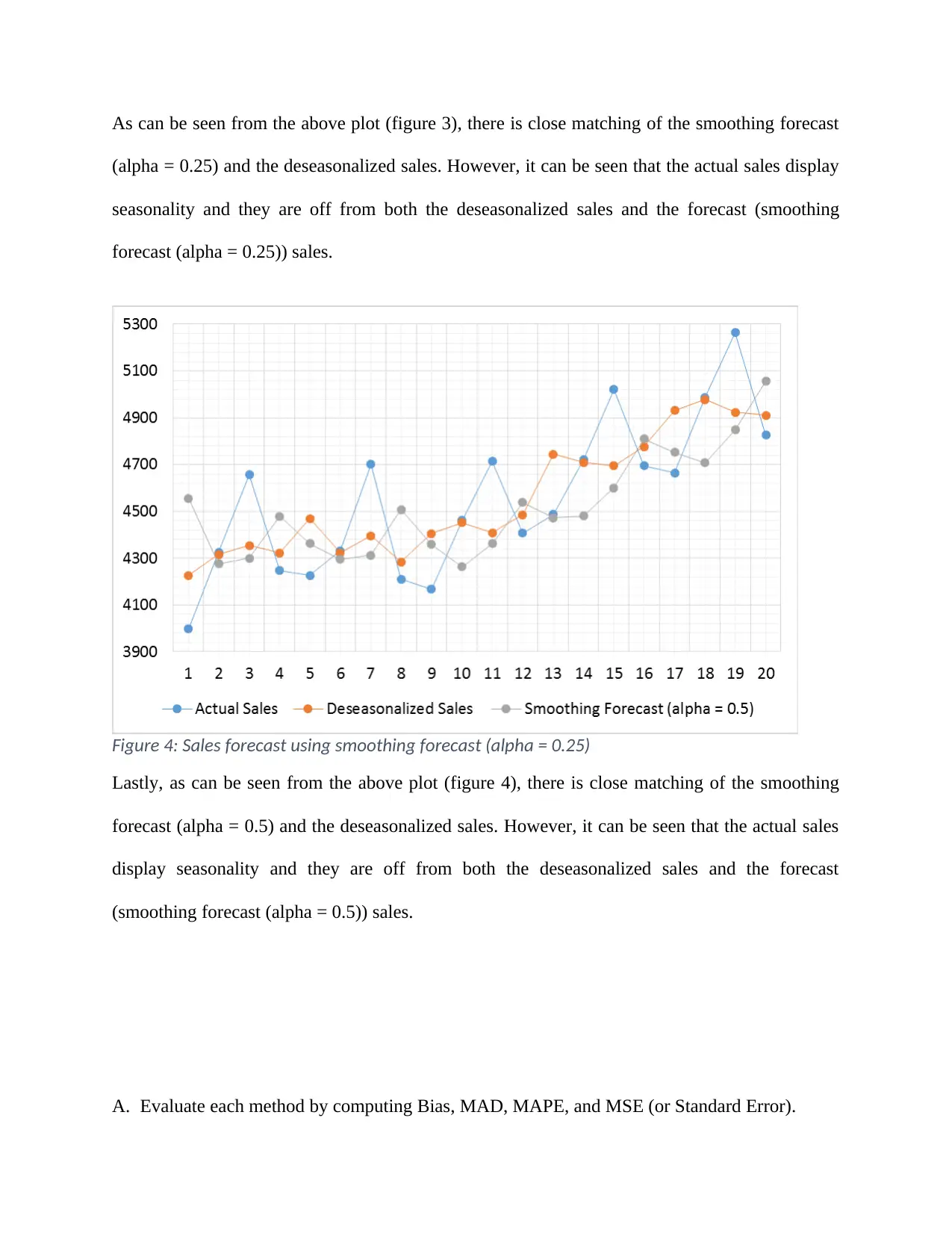
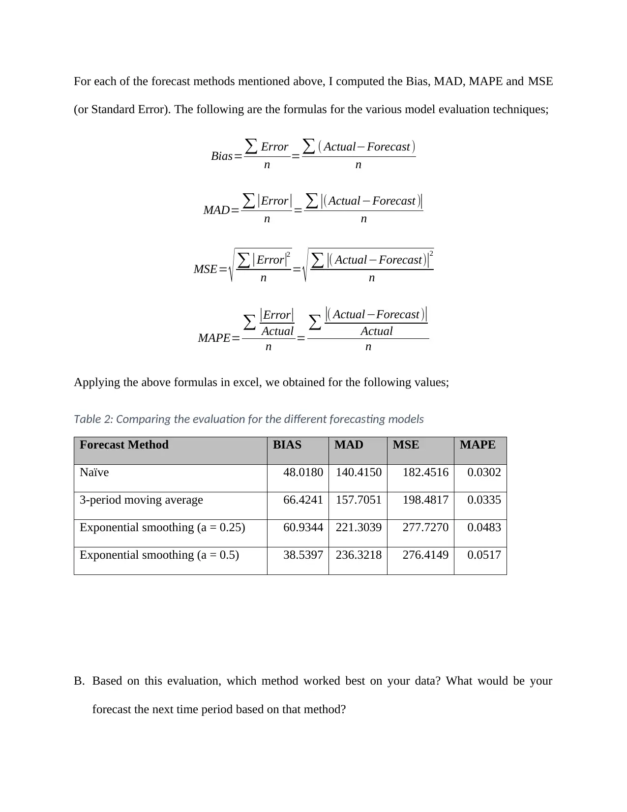
This report presents an analysis of time series data using various forecasting techniques, including Naive, Moving Average (3 period), and Exponential Smoothing (with alpha values of 0.25 and 0.5). The analysis involves deseasonalizing the data and comparing the actual sales with the forecasted sales generated by each method. The evaluation of each method is based on metrics such as Bias, MAD (Mean Absolute Deviation), MAPE (Mean Absolute Percentage Error), and MSE (Mean Squared Error). Based on these evaluations, the Naive method is identified as the most effective for the given dataset. The report also includes a commentary on the interpretation of Bias, MAD, and MAPE. The forecast for the next one year would be 4910.34.

Statistics Project
Student Name:
Student Number:
Date: 23rd February 2019

Introduction
Forecasting refers to the way toward making predictions of things (such as sales, yields,
convictions etc.) to come dependent on over a wide span of time data and most regularly by
analyzing the trends (Omalu, Shakir, Lindner, & Tayur, 2010). There are several methods that
can be used for forecasting and as analyst one is required to identify the most accurate or precise
method to perform the forecasting of the data (Munim & Schramm , 2017) This task sought to
work on time series data and forecast the data using the following four forecasting techniques:
 Naive
 Moving Average (3 period)
 Exponential Smoothing (Alpha = 0.25)
 Exponential Smoothing (Alpha = 0.5)
We considered quarterly sales data from 2012 to 2016 (representing 20 observations). The data is
presented in table 1 below;
Table 1: Quarterly sales data from 2012 to 2016
Year Quarter Actual Sales Year Quarter Actual Sales
2012 Q1 3998 2014 Q3 4714
2012 Q2 4325 2014 Q4 4408
2012 Q3 4656 2015 Q1 4487
2012 Q4 4248 2015 Q2 4720
2013 Q1 4227 2015 Q3 5021
2013 Q2 4332 2015 Q4 4695
2013 Q3 4701 2016 Q1 4664
2013 Q4 4210 2016 Q2 4988
2014 Q1 4167 2016 Q3 5264
2014 Q2 4462 2016 Q4 4826
Forecasting

Just before I estimated the forecast using the various forecasting models (Naïve, Moving
Average (3 period), Exponential Smoothing (Alpha = 0.25), Exponential Smoothing (Alpha =
0.5)), I ensured that I deseasonalized the data since it was a seasonal data. After deseasonalizing
the sales data, I computed the various forecasts requested based on the different forecasting
models.
The following graphs represents the plots of the actual sales, deseasonalized sales as well as the
forecast sales for the four forecasting methods applied.
Figure 1: Sales forecast using Naïve model
As can be seen from the above plot (figure 1), there is close matching of the naïve forecast and
the deseasonalized sales. However, it can be seen that the actual sales display seasonality and
they are off from both the deseasonalized sales and the forecast (naïve forecast) sales.

Figure 2: Sales forecast using 3-period moving average
As can be seen from the above plot (figure 2), there is close matching of the 3-period moving
average forecast and the deseasonalized sales. However, it can be seen that the actual sales
display seasonality and they are off from both the deseasonalized sales and the forecast (3-period
moving average forecast) sales.
Figure 3: Sales forecast using smoothing forecast (alpha = 0.25)

As can be seen from the above plot (figure 3), there is close matching of the smoothing forecast
(alpha = 0.25) and the deseasonalized sales. However, it can be seen that the actual sales display
seasonality and they are off from both the deseasonalized sales and the forecast (smoothing
forecast (alpha = 0.25)) sales.
Figure 4: Sales forecast using smoothing forecast (alpha = 0.25)
Lastly, as can be seen from the above plot (figure 4), there is close matching of the smoothing
forecast (alpha = 0.5) and the deseasonalized sales. However, it can be seen that the actual sales
display seasonality and they are off from both the deseasonalized sales and the forecast
(smoothing forecast (alpha = 0.5)) sales.
A. Evaluate each method by computing Bias, MAD, MAPE, and MSE (or Standard Error).

For each of the forecast methods mentioned above, I computed the Bias, MAD, MAPE and MSE
(or Standard Error). The following are the formulas for the various model evaluation techniques;
Bias=∑ Error
n =∑ ( Actual−Forecast )
n
MAD= ∑ |Error |
n = ∑ |(Actual−Forecast )|
n
MSE= √ ∑ |Error|2
n = √ ∑ |( Actual−Forecast)|2
n
MAPE=
∑ |Error|
Actual
n =
∑ |( Actual−Forecast )|
Actual
n
Applying the above formulas in excel, we obtained for the following values;
Table 2: Comparing the evaluation for the different forecasting models
Forecast Method BIAS MAD MSE MAPE
Naïve 48.0180 140.4150 182.4516 0.0302
3-period moving average 66.4241 157.7051 198.4817 0.0335
Exponential smoothing (a = 0.25) 60.9344 221.3039 277.7270 0.0483
Exponential smoothing (a = 0.5) 38.5397 236.3218 276.4149 0.0517
B. Based on this evaluation, which method worked best on your data? What would be your
forecast the next time period based on that method?

Answer
Based on the above evaluation, Naïve method of forecasting worked best for the given sales
data. This is based on the fact that all the evaluation parameters (Bias, MAD, MSE and
MAPE) were lowest for the Naïve method. The forecast for the next one year would be
4910.34.
C. Write a brief general commentary on Bias, MAD, and MAPE describing what they mean
(i.e., their interpretation).
Answer
Bias refers to the average of the differences obtained between the actual data and the forecast
data. The smaller the bias of a given forecast model, the better the model is while a large bias
indicates that the difference between the actual data and the forecast data is large and as such
the forecast values are not close to the actual values.
MAD on the other hand refers to the average of the absolute differences obtained between
the actual data and the forecast data. Just like the case of bias, the smaller the value of the
MAD, the better the model is while a large value of MAD indicates that the absolute
difference between the actual data and the forecast data is large and as such the forecast
values are not close to the actual values.
Lastly MAPE refers to the mean absolute percentage error where the absolute error is divided
by the actual sales and then the average is obtained. Just like in the two other evaluations
methods, the smaller the value of the MAPE, the better the model in forecasting the data.
References

Munim, Z. H., & Schramm , H.-J. (2017). Forecasting container shipping freight rates for the Far
East – Northern Europe trade lane. Maritime Economics & Logistics, 19(1), 106–125.
doi:10.1057/s41278-016-0051-7
Omalu, B. I., Shakir, A. M., Lindner, J. L., & Tayur, S. R. (2010). Forecasting as an Operations
Management Tool in a Medical Examiner's Office. Journal of Health Management, 9(5),
75–84. doi:10.1177/097206340700900105