Econometrics: Time Series Analysis of Monetary Policy VAR Model

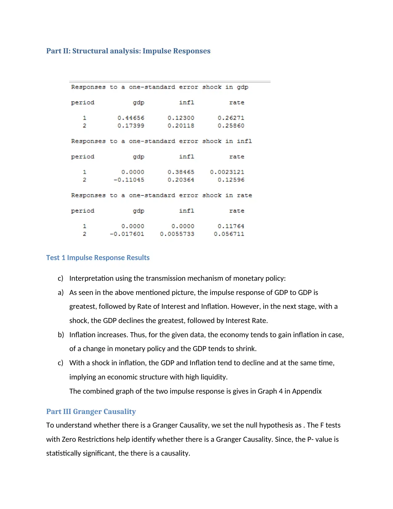
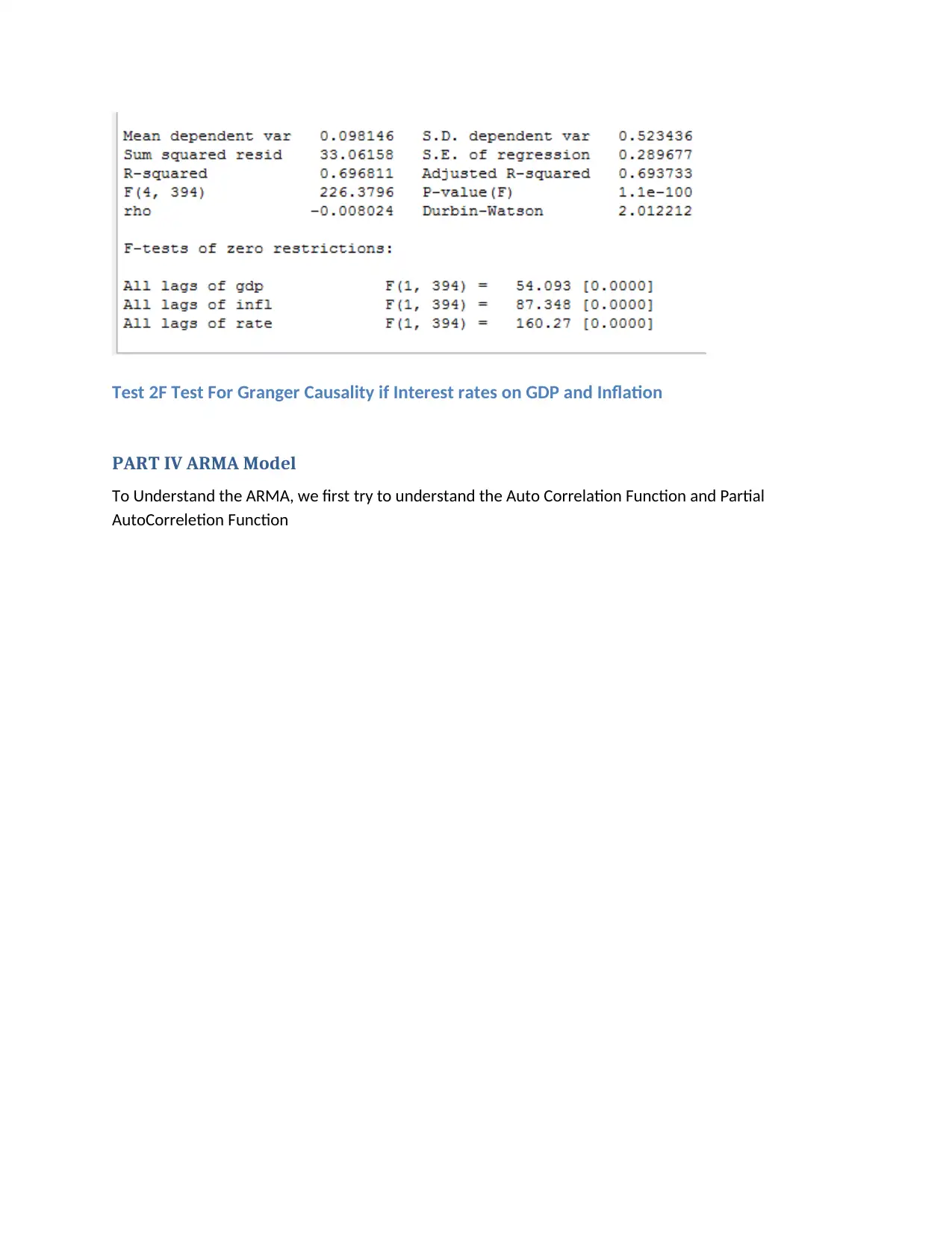
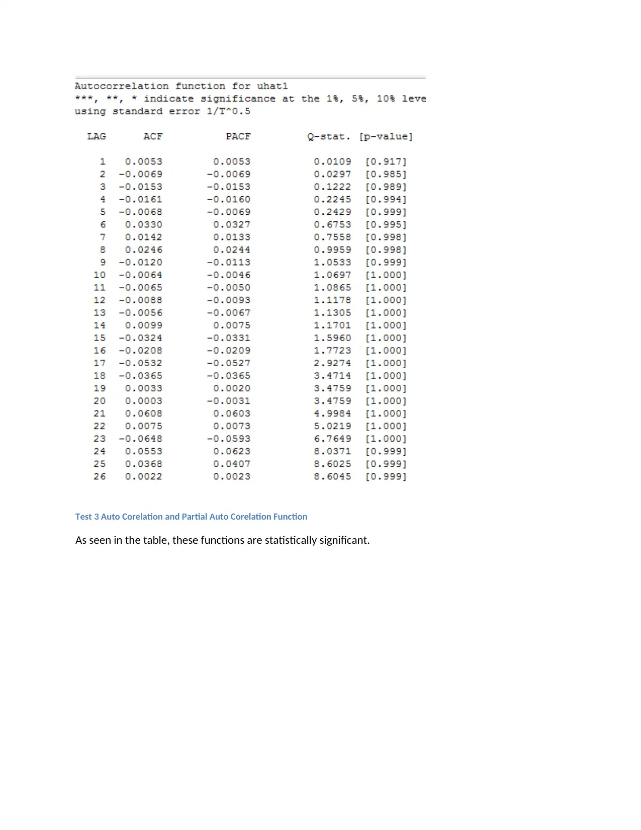
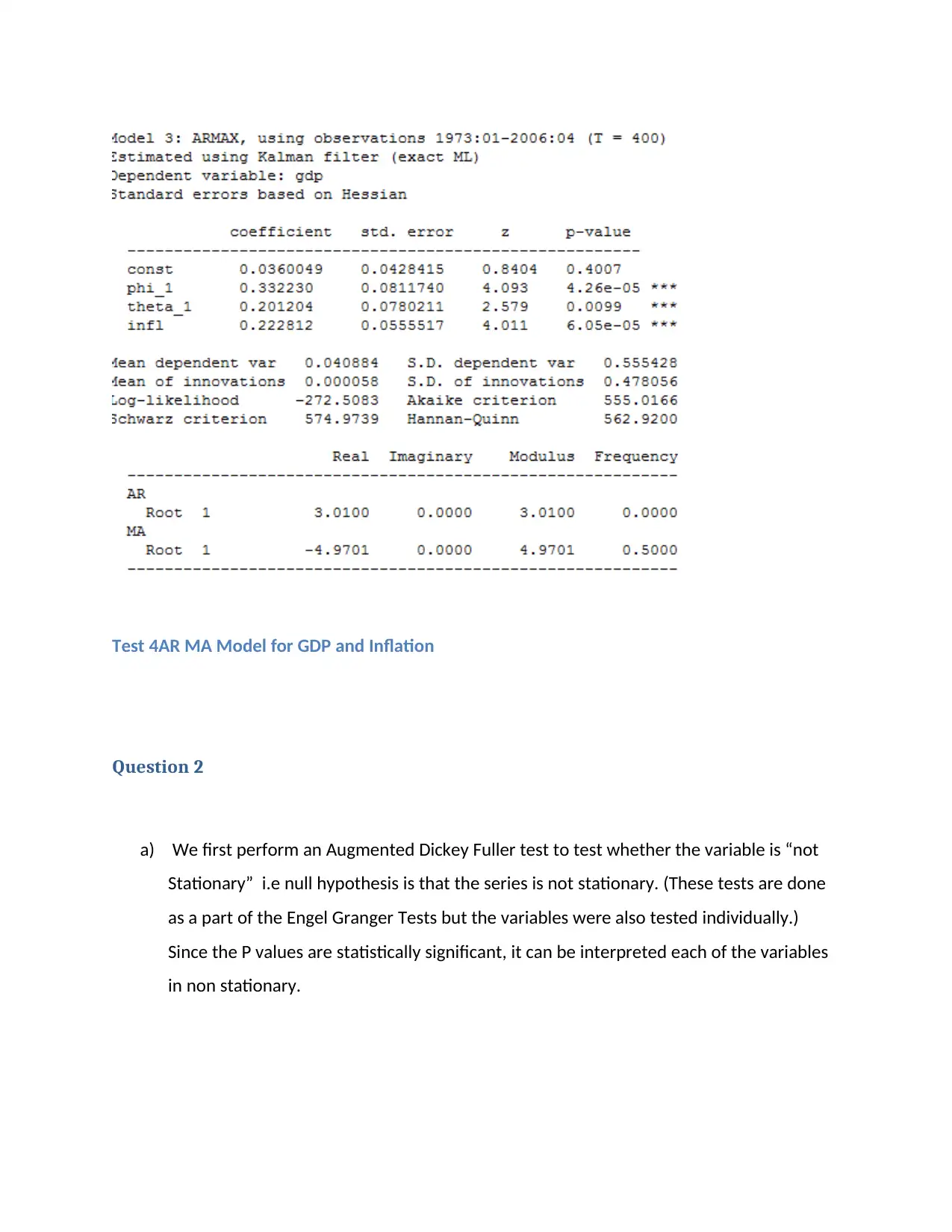
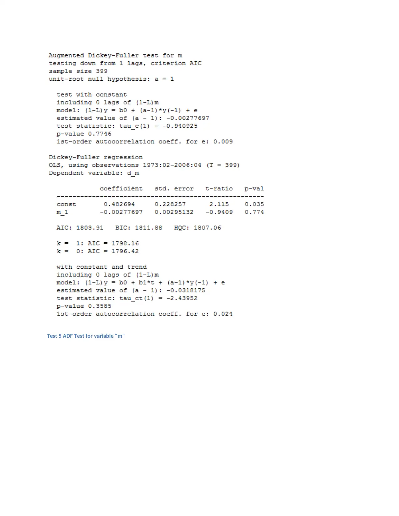
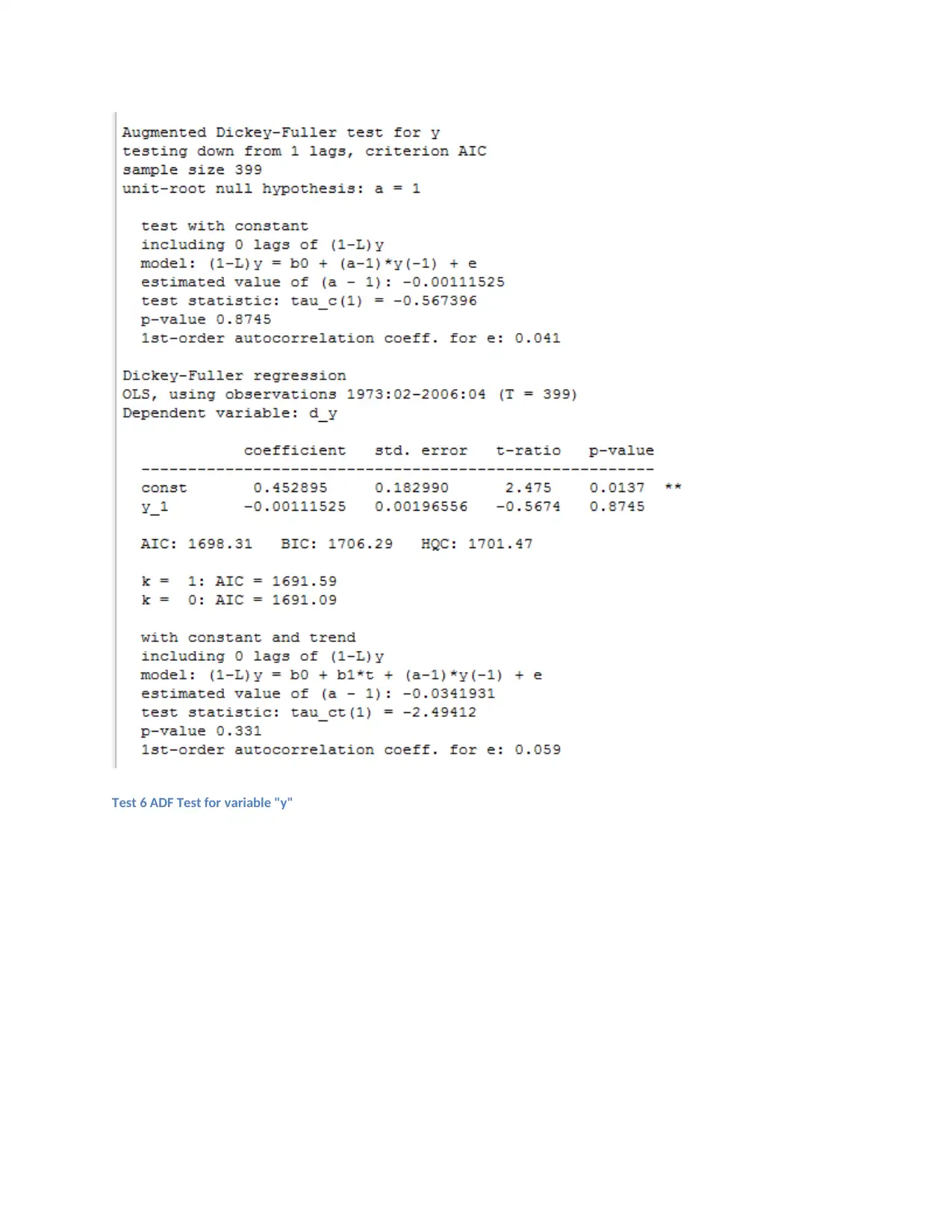
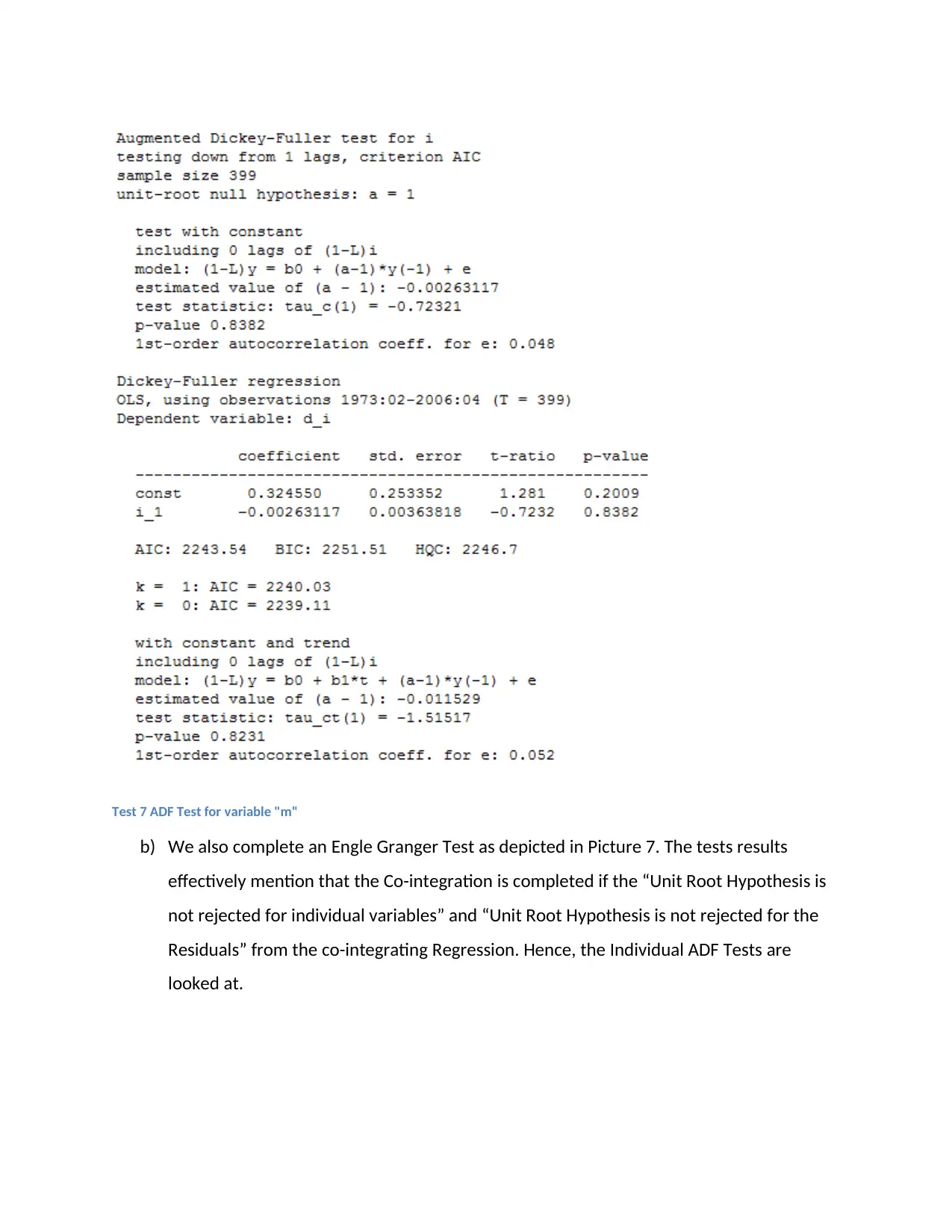
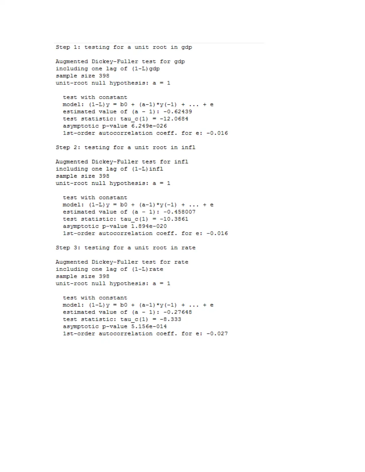
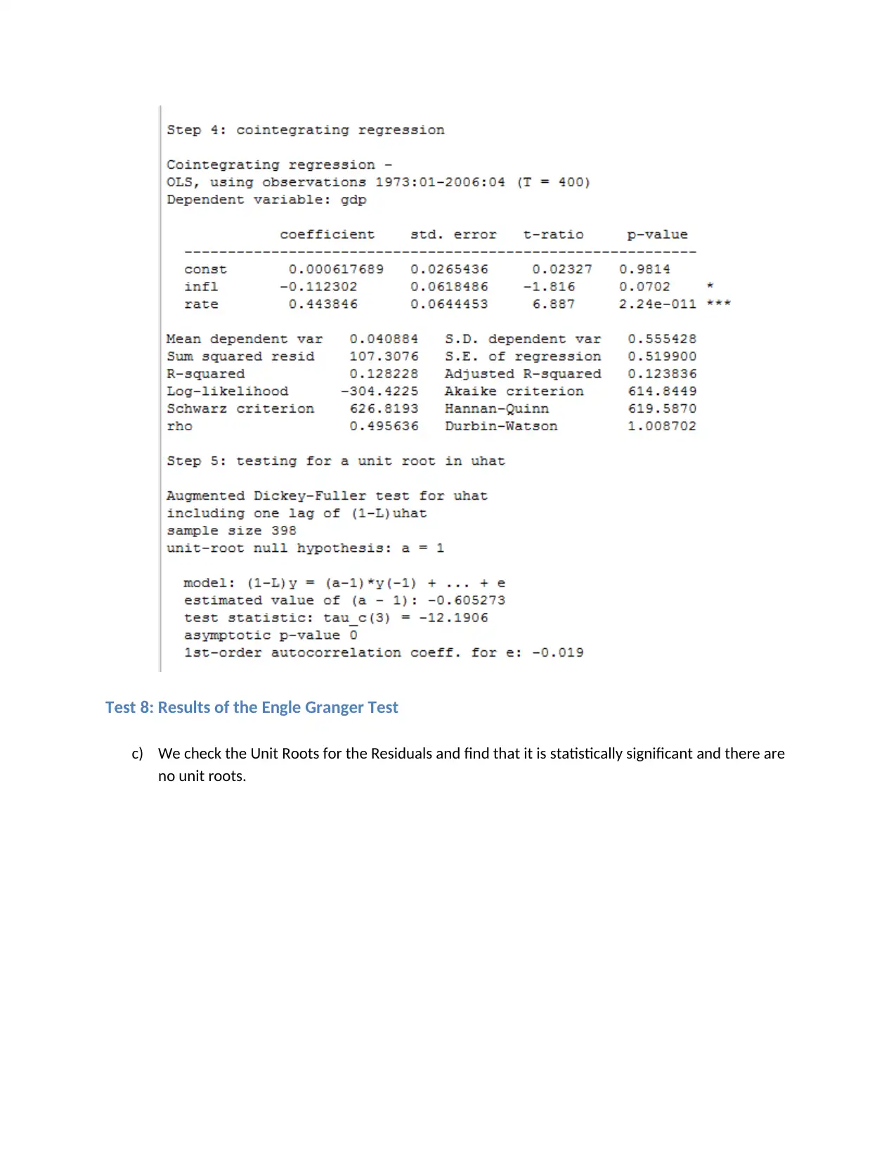
This assignment provides a comprehensive analysis of monetary policy transmission using a Vector Autoregression (VAR) model. It begins by assessing the stationarity of the time series data through visual inspection and formal tests like the Augmented Dickey-Fuller (ADF) and KPSS tests. The VAR model is constructed with appropriate lag selection, followed by structural analysis using impulse response functions to understand the dynamic interactions between GDP growth rate, inflation rate, and policy interest rate. Granger causality tests are performed to determine the causal relationships between the variables. Additionally, an ARMA model is employed, and cointegration tests, such as the Engle-Granger test, are conducted to assess the long-run equilibrium relationships between variables. The analysis includes interpretations of the impulse responses, Granger causality test results, and cointegration test outcomes, providing insights into the transmission mechanism of monetary policy.

qwertyuiopasdfghjklzxcvbnmqwertyui
opasdfghjklzxcvbnmqwertyuiopasdfgh
jklzxcvbnmqwertyuiopasdfghjklzxcvb
nmqwertyuiopasdfghjklzxcvbnmqwer
tyuiopasdfghjklzxcvbnmqwertyuiopas
dfghjklzxcvbnmqwertyuiopasdfghjklzx
cvbnmqwertyuiopasdfghjklzxcvbnmq
wertyuiopasdfghjklzxcvbnmqwertyuio
pasdfghjklzxcvbnmqwertyuiopasdfghj
klzxcvbnmqwertyuiopasdfghjklzxcvbn
mqwertyuiopasdfghjklzxcvbnmqwerty
uiopasdfghjklzxcvbnmqwertyuiopasdf
ghjklzxcvbnmqwertyuiopasdfghjklzxc
vbnmqwertyuiopasdfghjklzxcvbnmrty
uiopasdfghjklzxcvbnmqwertyuiopasdf
ghjklzxcvbnmqwertyuiopasdfghjklzxc
Time Series Analysis,
December 2017
[Pick the date]
Com

Question 1
Part I : Model
a) In order to complete the model, we first found the number of lags to be included in the
analysis. To Do so, we took a time series analysis. All variables were taken for this
analysis. We have taken maximum lag as 1 since the data is given as yearly. First, an
informal analysis of stationarity was conducted by looking at the time series plot. All the
variables are around the mean, implying that the variables are stationary. (See Appendix
: Graphs 1-3) We also identified if the data has a constant and no trend.
b) Next we conducted a formal Analysis of Unit roots using the Advanced Dicky Fuller Test
and KPSS tests to test the non-stationarity and stationarity.
The OLS Estimates are as follows
Equation 1: gdp
coefficient std. error t-ratio p-value
------------------------------------------------------------
const 0.0453425 0.0455777 0.9948 0.3204
gdp_1 0.556470 0.0434717 12.80 1.30e-031 ***
infl_1 −0.286246 0.0538757 −5.313 1.81e-07 ***
rate_1 −0.149610 0.0590711 −2.533 0.0117 **
time −1.58047e-05 0.000195764 −0.08073 0.9357
Equation 2: infl

coefficient std. error t-ratio p-value
-----------------------------------------------------------
const 0.0310928 0.0412172 0.7544 0.4511
gdp_1 0.276891 0.0393126 7.043 8.42e-012 ***
infl_1 0.529129 0.0487213 10.86 3.27e-024 ***
rate_1 0.0473744 0.0534196 0.8868 0.3757
time −0.000165645 0.000177035 −0.9357 0.3500
Equation 3: rate
coefficient std. error t-ratio p-value
----------------------------------------------------------
const 0.0314197 0.0293796 1.069 0.2855
gdp_1 0.206096 0.0280220 7.355 1.12e-012 ***
infl_1 0.324573 0.0347285 9.346 6.89e-019 ***
rate_1 0.482056 0.0380774 12.66 4.68e-031 ***
time 1.40105e-05 0.000126190 0.1110 0.9117

Part II: Structural analysis: Impulse Responses
Test 1 Impulse Response Results
c) Interpretation using the transmission mechanism of monetary policy:
a) As seen in the above mentioned picture, the impulse response of GDP to GDP is
greatest, followed by Rate of Interest and Inflation. However, in the next stage, with a
shock, the GDP declines the greatest, followed by Interest Rate.
b) Inflation increases. Thus, for the given data, the economy tends to gain inflation in case,
of a change in monetary policy and the GDP tends to shrink.
c) With a shock in inflation, the GDP and Inflation tend to decline and at the same time,
implying an economic structure with high liquidity.
The combined graph of the two impulse response is gives in Graph 4 in Appendix
Part III Granger Causality
To understand whether there is a Granger Causality, we set the null hypothesis as . The F tests
with Zero Restrictions help identify whether there is a Granger Causality. Since, the P- value is
statistically significant, the there is a causality.

Test 2F Test For Granger Causality if Interest rates on GDP and Inflation
PART IV ARMA Model
To Understand the ARMA, we first try to understand the Auto Correlation Function and Partial
AutoCorreletion Function

Test 3 Auto Corelation and Partial Auto Corelation Function
As seen in the table, these functions are statistically significant.

Test 4AR MA Model for GDP and Inflation
Question 2
a) We first perform an Augmented Dickey Fuller test to test whether the variable is “not
Stationary” i.e null hypothesis is that the series is not stationary. (These tests are done
as a part of the Engel Granger Tests but the variables were also tested individually.)
Since the P values are statistically significant, it can be interpreted each of the variables
in non stationary.

Test 5 ADF Test for variable "m"

Test 6 ADF Test for variable "y"

Test 7 ADF Test for variable "m"
b) We also complete an Engle Granger Test as depicted in Picture 7. The tests results
effectively mention that the Co-integration is completed if the “Unit Root Hypothesis is
not rejected for individual variables” and “Unit Root Hypothesis is not rejected for the
Residuals” from the co-integrating Regression. Hence, the Individual ADF Tests are
looked at.

Test 8: Results of the Engle Granger Test
c) We check the Unit Roots for the Residuals and find that it is statistically significant and there are
no unit roots.