Time Series & Regression Modeling

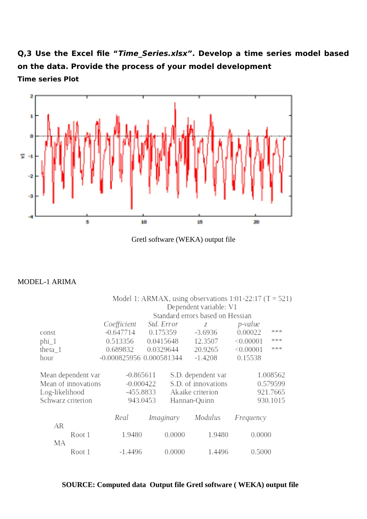
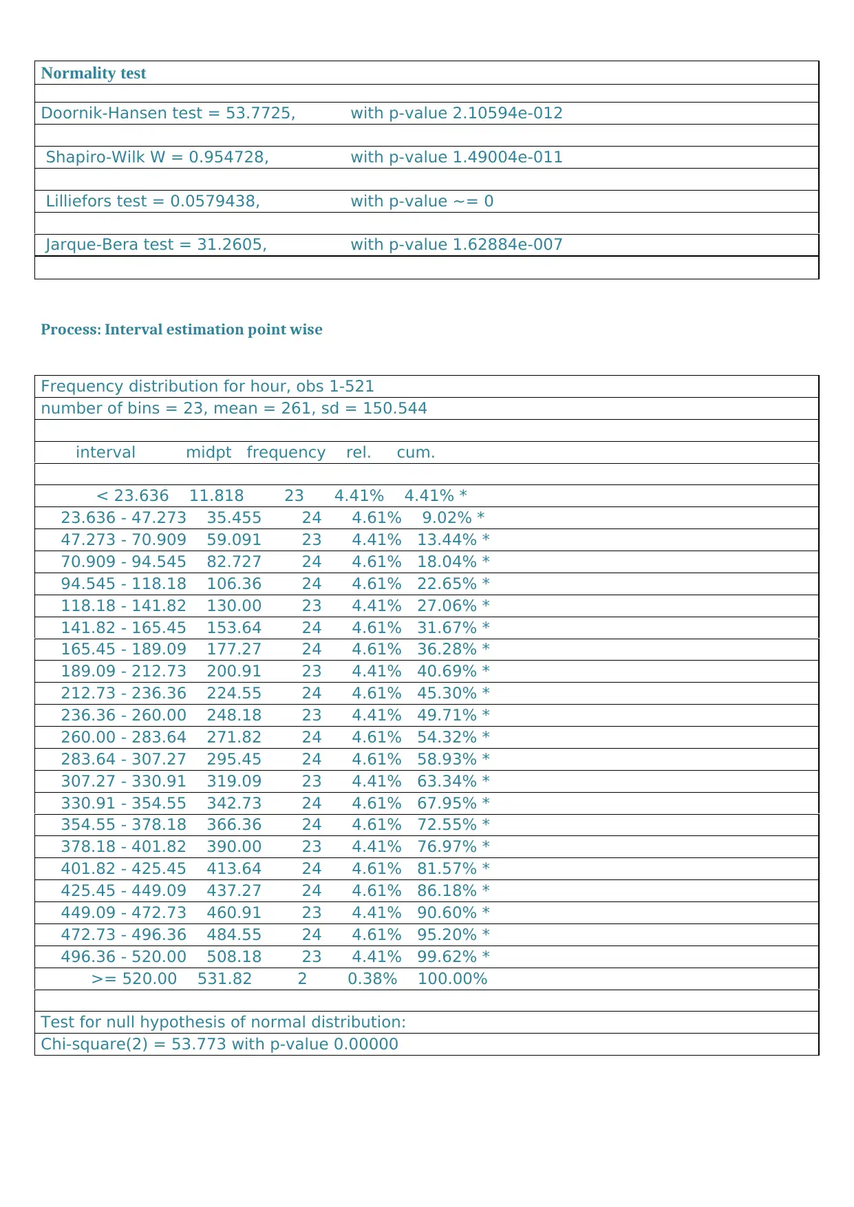
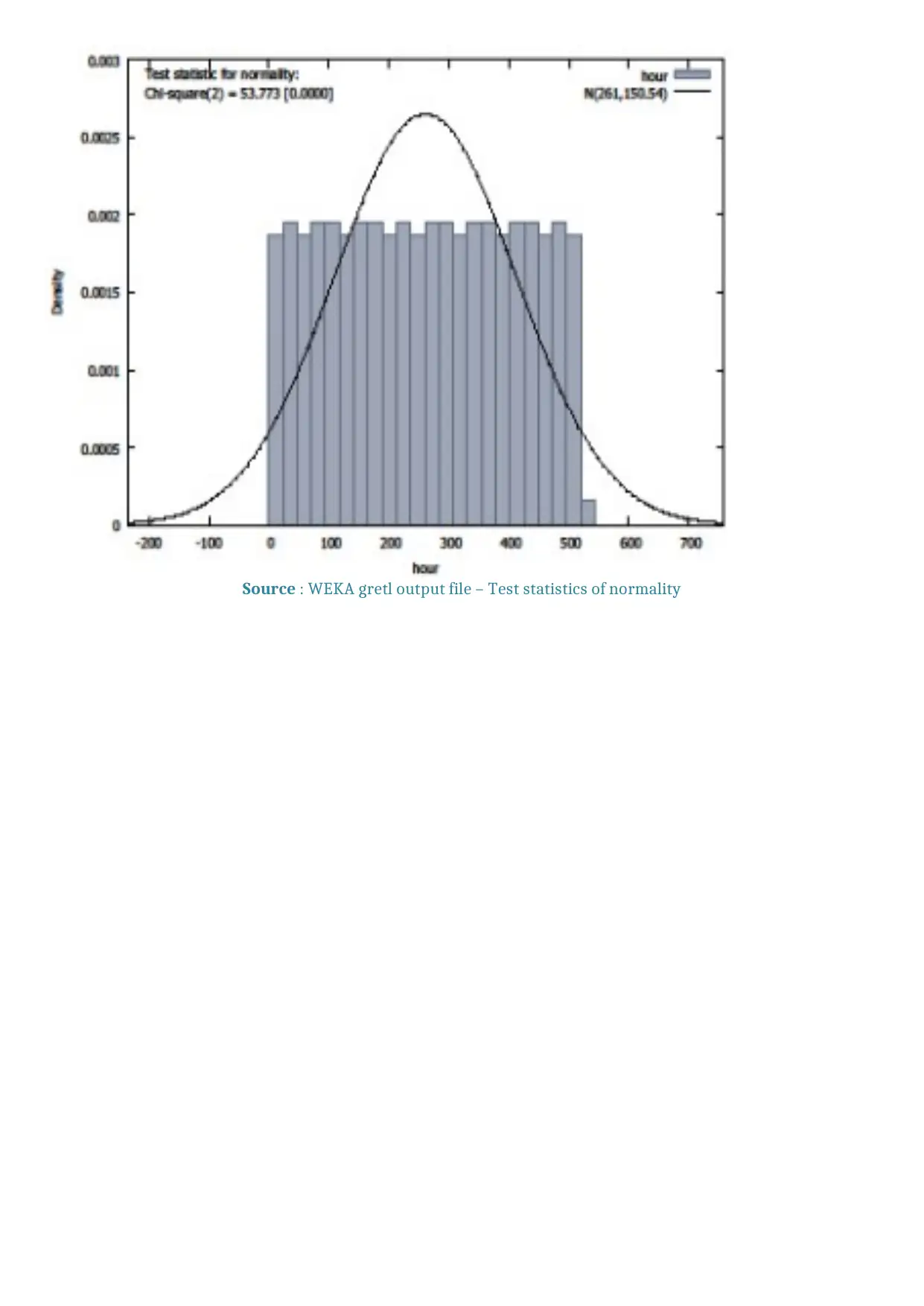
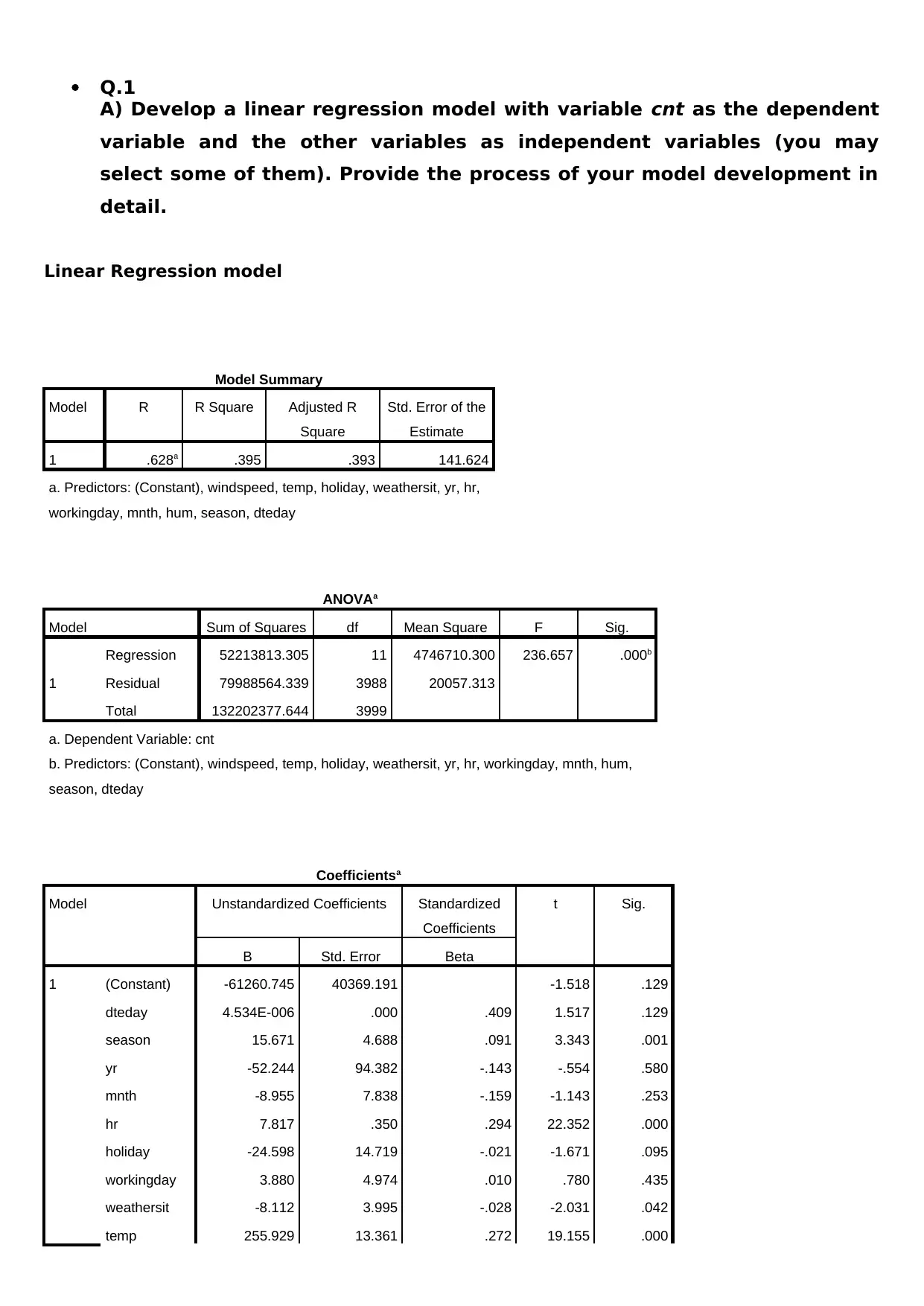
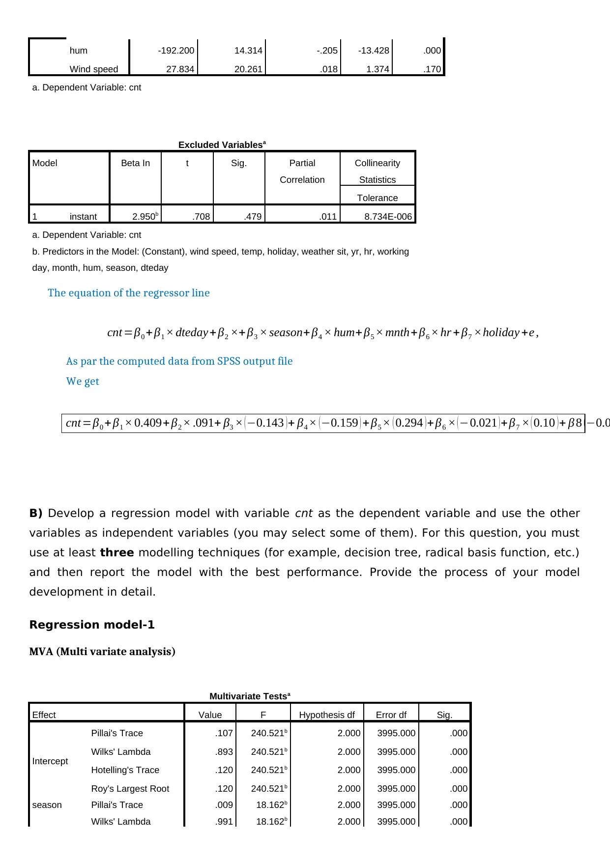
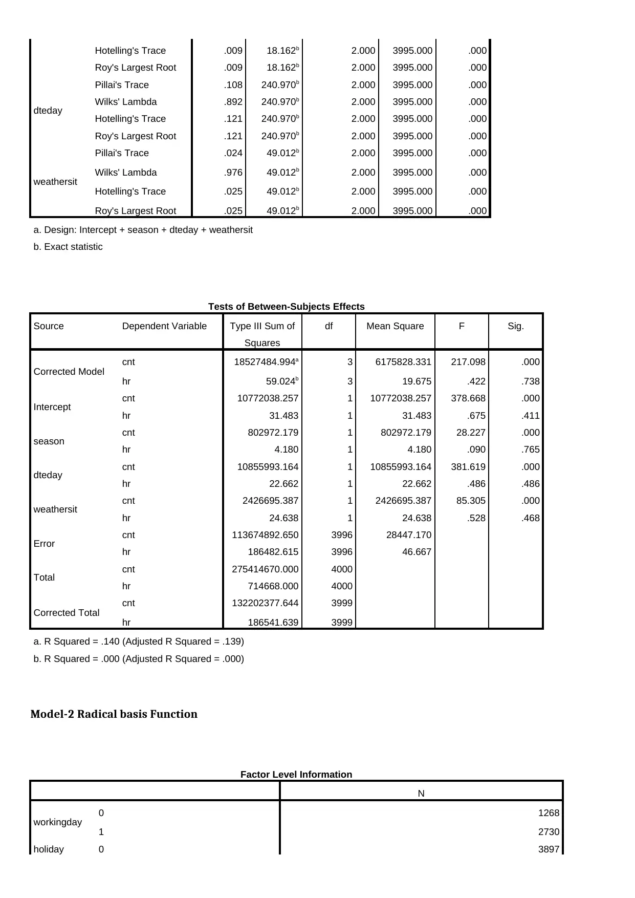
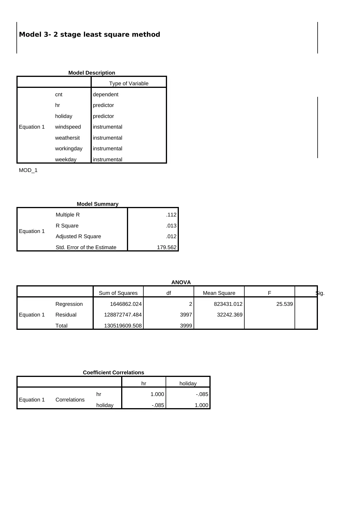
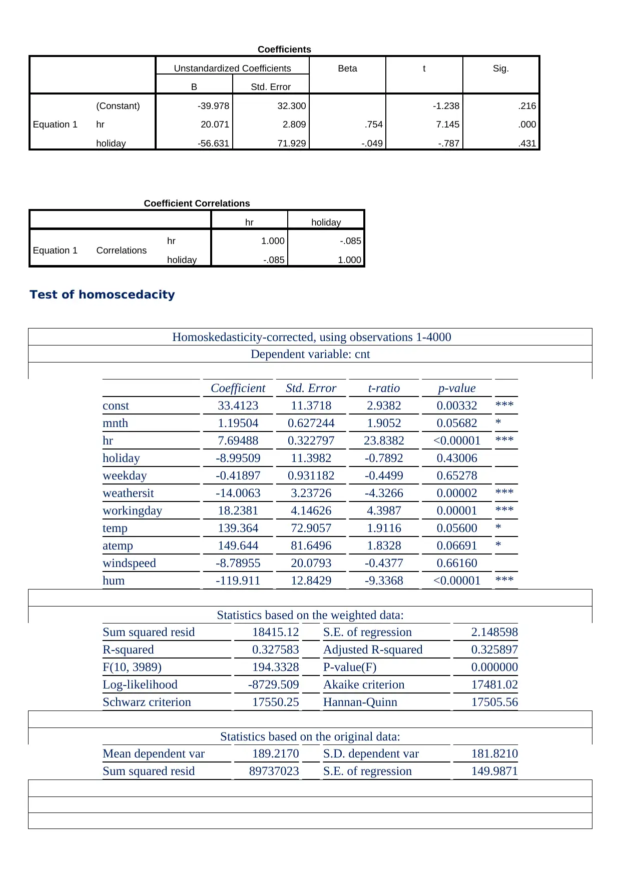
This practical assignment involves developing several statistical models using a provided Excel file ('Time_Series.xlsx'). The first part focuses on building a time series model, detailing the process including time series plots and normality tests (Doornik-Hansen, Shapiro-Wilk, Lilliefors, Jarque-Bera) using Gretl or WEKA software. The second part requires developing a linear regression model with 'cnt' as the dependent variable and other variables as independent variables, documenting the model development process, including ANOVA and coefficient analysis. The third part necessitates employing at least three different regression modeling techniques (e.g., decision tree, radical basis function, 2-stage least squares) to predict 'cnt', selecting the best-performing model. Finally, a logistic regression model is to be built with 'Y' as the dependent variable and other variables as independent variables, along with a classification model using at least three techniques (e.g., k-means clustering, general log-linear model, curve estimation) to classify 'Y'. The assignment requires detailed documentation of the model development process for each model, including relevant statistical outputs and interpretations. A mapping table is provided for submitting the logistic regression model results in an MS Excel file.

Q,3 Use the Excel file “Time_Series.xlsx”. Develop a time series model based
on the data. Provide the process of your model development
Time series Plot
Gretl software (WEKA) output file
MODEL-1 ARIMA
SOURCE: Computed data Output file Gretl software ( WEKA) output file

Normality test
Doornik-Hansen test = 53.7725, with p-value 2.10594e-012
Shapiro-Wilk W = 0.954728, with p-value 1.49004e-011
Lilliefors test = 0.0579438, with p-value ~= 0
Jarque-Bera test = 31.2605, with p-value 1.62884e-007
Process: Interval estimation point wise
Frequency distribution for hour, obs 1-521
number of bins = 23, mean = 261, sd = 150.544
interval midpt frequency rel. cum.
< 23.636 11.818 23 4.41% 4.41% *
23.636 - 47.273 35.455 24 4.61% 9.02% *
47.273 - 70.909 59.091 23 4.41% 13.44% *
70.909 - 94.545 82.727 24 4.61% 18.04% *
94.545 - 118.18 106.36 24 4.61% 22.65% *
118.18 - 141.82 130.00 23 4.41% 27.06% *
141.82 - 165.45 153.64 24 4.61% 31.67% *
165.45 - 189.09 177.27 24 4.61% 36.28% *
189.09 - 212.73 200.91 23 4.41% 40.69% *
212.73 - 236.36 224.55 24 4.61% 45.30% *
236.36 - 260.00 248.18 23 4.41% 49.71% *
260.00 - 283.64 271.82 24 4.61% 54.32% *
283.64 - 307.27 295.45 24 4.61% 58.93% *
307.27 - 330.91 319.09 23 4.41% 63.34% *
330.91 - 354.55 342.73 24 4.61% 67.95% *
354.55 - 378.18 366.36 24 4.61% 72.55% *
378.18 - 401.82 390.00 23 4.41% 76.97% *
401.82 - 425.45 413.64 24 4.61% 81.57% *
425.45 - 449.09 437.27 24 4.61% 86.18% *
449.09 - 472.73 460.91 23 4.41% 90.60% *
472.73 - 496.36 484.55 24 4.61% 95.20% *
496.36 - 520.00 508.18 23 4.41% 99.62% *
>= 520.00 531.82 2 0.38% 100.00%
Test for null hypothesis of normal distribution:
Chi-square(2) = 53.773 with p-value 0.00000

Source : WEKA gretl output file – Test statistics of normality

 Q.1
A) Develop a linear regression model with variable cnt as the dependent
variable and the other variables as independent variables (you may
select some of them). Provide the process of your model development in
detail.
Linear Regression model
Model Summary
Model R R Square Adjusted R
Square
Std. Error of the
Estimate
1 .628a .395 .393 141.624
a. Predictors: (Constant), windspeed, temp, holiday, weathersit, yr, hr,
workingday, mnth, hum, season, dteday
ANOVAa
Model Sum of Squares df Mean Square F Sig.
1
Regression 52213813.305 11 4746710.300 236.657 .000b
Residual 79988564.339 3988 20057.313
Total 132202377.644 3999
a. Dependent Variable: cnt
b. Predictors: (Constant), windspeed, temp, holiday, weathersit, yr, hr, workingday, mnth, hum,
season, dteday
Coefficientsa
Model Unstandardized Coefficients Standardized
Coefficients
t Sig.
B Std. Error Beta
1 (Constant) -61260.745 40369.191 -1.518 .129
dteday 4.534E-006 .000 .409 1.517 .129
season 15.671 4.688 .091 3.343 .001
yr -52.244 94.382 -.143 -.554 .580
mnth -8.955 7.838 -.159 -1.143 .253
hr 7.817 .350 .294 22.352 .000
holiday -24.598 14.719 -.021 -1.671 .095
workingday 3.880 4.974 .010 .780 .435
weathersit -8.112 3.995 -.028 -2.031 .042
temp 255.929 13.361 .272 19.155 .000

hum -192.200 14.314 -.205 -13.428 .000
Wind speed 27.834 20.261 .018 1.374 .170
a. Dependent Variable: cnt
Excluded Variablesa
Model Beta In t Sig. Partial
Correlation
Collinearity
Statistics
Tolerance
1 instant 2.950b .708 .479 .011 8.734E-006
a. Dependent Variable: cnt
b. Predictors in the Model: (Constant), wind speed, temp, holiday, weather sit, yr, hr, working
day, month, hum, season, dteday
The equation of the regressor line
cnt =β0 + β1 × dteday+ β2 ×+ β3 × season+ β4 × hum+ β5 × mnth+β6 × hr + β7 ×holiday +e ,
As par the computed data from SPSS output file
We get
cnt=β0 + β1 × 0.409+ β2 × .091+ β3 × ( −0.143 ) + β4 × ( −0.159 ) + β5 × ( 0.294 ) + β6 × ( −0.021 ) + β7 × ( 0.10 ) + β 8 ( −0.0
B) Develop a regression model with variable cnt as the dependent variable and use the other
variables as independent variables (you may select some of them). For this question, you must
use at least three modelling techniques (for example, decision tree, radical basis function, etc.)
and then report the model with the best performance. Provide the process of your model
development in detail.
Regression model-1
MVA (Multi variate analysis)
Multivariate Testsa
Effect Value F Hypothesis df Error df Sig.
Intercept
Pillai's Trace .107 240.521b 2.000 3995.000 .000
Wilks' Lambda .893 240.521b 2.000 3995.000 .000
Hotelling's Trace .120 240.521b 2.000 3995.000 .000
Roy's Largest Root .120 240.521b 2.000 3995.000 .000
season Pillai's Trace .009 18.162b 2.000 3995.000 .000
Wilks' Lambda .991 18.162b 2.000 3995.000 .000

Hotelling's Trace .009 18.162b 2.000 3995.000 .000
Roy's Largest Root .009 18.162b 2.000 3995.000 .000
dteday
Pillai's Trace .108 240.970b 2.000 3995.000 .000
Wilks' Lambda .892 240.970b 2.000 3995.000 .000
Hotelling's Trace .121 240.970b 2.000 3995.000 .000
Roy's Largest Root .121 240.970b 2.000 3995.000 .000
weathersit
Pillai's Trace .024 49.012b 2.000 3995.000 .000
Wilks' Lambda .976 49.012b 2.000 3995.000 .000
Hotelling's Trace .025 49.012b 2.000 3995.000 .000
Roy's Largest Root .025 49.012b 2.000 3995.000 .000
a. Design: Intercept + season + dteday + weathersit
b. Exact statistic
Tests of Between-Subjects Effects
Source Dependent Variable Type III Sum of
Squares
df Mean Square F Sig.
Corrected Model cnt 18527484.994a 3 6175828.331 217.098 .000
hr 59.024b 3 19.675 .422 .738
Intercept cnt 10772038.257 1 10772038.257 378.668 .000
hr 31.483 1 31.483 .675 .411
season cnt 802972.179 1 802972.179 28.227 .000
hr 4.180 1 4.180 .090 .765
dteday cnt 10855993.164 1 10855993.164 381.619 .000
hr 22.662 1 22.662 .486 .486
weathersit cnt 2426695.387 1 2426695.387 85.305 .000
hr 24.638 1 24.638 .528 .468
Error cnt 113674892.650 3996 28447.170
hr 186482.615 3996 46.667
Total cnt 275414670.000 4000
hr 714668.000 4000
Corrected Total cnt 132202377.644 3999
hr 186541.639 3999
a. R Squared = .140 (Adjusted R Squared = .139)
b. R Squared = .000 (Adjusted R Squared = .000)
Model-2 Radical basis Function
Factor Level Information
N
workingday 0 1268
1 2730
holiday 0 3897

1 101
yr 0 2163
1 1835
Dependent Variable: cnt
Variance Estimatesa
Component Estimate
Var(workingday) -57.623b
Var(workingday * holiday) .000c
Var(workingday * yr) 205.487
Var(workingday * holiday * yr) .000c
Var(Error) 14925.477
Dependent Variable: cnt
Method: Minimum Norm Quadratic Unbiased Estimation (Weight = 1 for Random Effects and Residual)
a. Weighted Analysis - Weighted by hum
b. For the ANOVA and MINQUE methods, negative variance component estimates may occur. Some possible reasons for
their occurrence are: (a) the specified model is not the correct model, or (b) the true value of the variance equals zero.
Model 3- 2 stage least square method
Model Description
Type of Variable
Equation 1
cnt dependent
hr predictor
holiday predictor
windspeed instrumental
weathersit instrumental
workingday instrumental
weekday instrumental
MOD_1
Model Summary
Equation 1
Multiple R .112
R Square .013
Adjusted R Square .012
Std. Error of the Estimate 179.562
ANOVA
Sum of Squares df Mean Square F Sig.
Equation 1
Regression 1646862.024 2 823431.012 25.539
Residual 128872747.484 3997 32242.369
Total 130519609.508 3999
Coefficient Correlations
hr holiday
Equation 1 Correlations hr 1.000 -.085
holiday -.085 1.000

Coefficients
Unstandardized Coefficients Beta t Sig.
B Std. Error
Equation 1
(Constant) -39.978 32.300 -1.238 .216
hr 20.071 2.809 .754 7.145 .000
holiday -56.631 71.929 -.049 -.787 .431
Coefficient Correlations
hr holiday
Equation 1 Correlations hr 1.000 -.085
holiday -.085 1.000
Test of homoscedacity
Homoskedasticity-corrected, using observations 1-4000
Dependent variable: cnt
Coefficient Std. Error t-ratio p-value
const 33.4123 11.3718 2.9382 0.00332 ***
mnth 1.19504 0.627244 1.9052 0.05682 *
hr 7.69488 0.322797 23.8382 <0.00001 ***
holiday -8.99509 11.3982 -0.7892 0.43006
weekday -0.41897 0.931182 -0.4499 0.65278
weathersit -14.0063 3.23726 -4.3266 0.00002 ***
workingday 18.2381 4.14626 4.3987 0.00001 ***
temp 139.364 72.9057 1.9116 0.05600 *
atemp 149.644 81.6496 1.8328 0.06691 *
windspeed -8.78955 20.0793 -0.4377 0.66160
hum -119.911 12.8429 -9.3368 <0.00001 ***
Statistics based on the weighted data:
Sum squared resid 18415.12 S.E. of regression 2.148598
R-squared 0.327583 Adjusted R-squared 0.325897
F(10, 3989) 194.3328 P-value(F) 0.000000
Log-likelihood -8729.509 Akaike criterion 17481.02
Schwarz criterion 17550.25 Hannan-Quinn 17505.56
Statistics based on the original data:
Mean dependent var 189.2170 S.D. dependent var 181.8210
Sum squared resid 89737023 S.E. of regression 149.9871

Homoscedacity based on cnt( non linear plot)
Source : WEKA gretl output file
Q,2
A)Develop a logistic regression model with variable Y as the dependent variable and
the other variables as independent variables (you may select some of them). Provide
the process of your model development in detail.
Logistic Regression model
Assuming that following model was adopted
log( p
1− p )=β0 + β1 × X 1+β2 × X 2+ β3 × X 3+ β4 × X 4+ β5 × X 5+ β6 × X 6+ β7 × X 7+e ,On uploading the data in
the spss , the following results were obtained.
Data Information

N
Cases
Valid 5550
Missing 0
Weighted Valid 5550
Cells
Defined Cells 220
Structural Zeros 0
Sampling Zeros 148
Categories
Y 2
X8 11
X10 10
Convergence Informationa,b
Maximum Number of
Iterations
20
Converge Tolerance .00100
Final Maximum Absolute
Difference
7.39611E-009c
Final Maximum Relative
Difference
7.53116E-010
Number of Iterations 18
a. Model: Multinomial Logit
b. Design: Constant + Y + Y * X10 + Y * X13 + Y
* X14 + Y * X15
c. The iteration converged because the
maximum absolute changes of parameter
estimates is less than the specified convergence
criterion.
Goodness-of-Fit Testsa,b
Value df Sig.
Likelihood Ratio 111.758 94 .102
Pearson Chi-Square 140.788 94 .001
a. Model: Multinomial Logit
b. Design: Constant + Y + Y * X10 + Y * X13 + Y * X14 + Y *
X15
Analysis of Dispersiona,b
Entropy Concentration df
Model 200.601 163.233 15
Residual 2768.627 1781.380 5534
Total 2969.227 1944.613 5549
a. Model: Multinomial Logit

b. Design: Constant + Y + Y * X10 + Y * X13 + Y * X14
+ Y * X15
Measure of Associationa,b
Entropy .068
Concentration .084
a. Model: Multinomial Logit
b. Design: Constant + Y + Y *
X10 + Y * X13 + Y * X14 + Y *
X15