University Top Dynamics Assignment 2 Solution: Mechanical Engineering

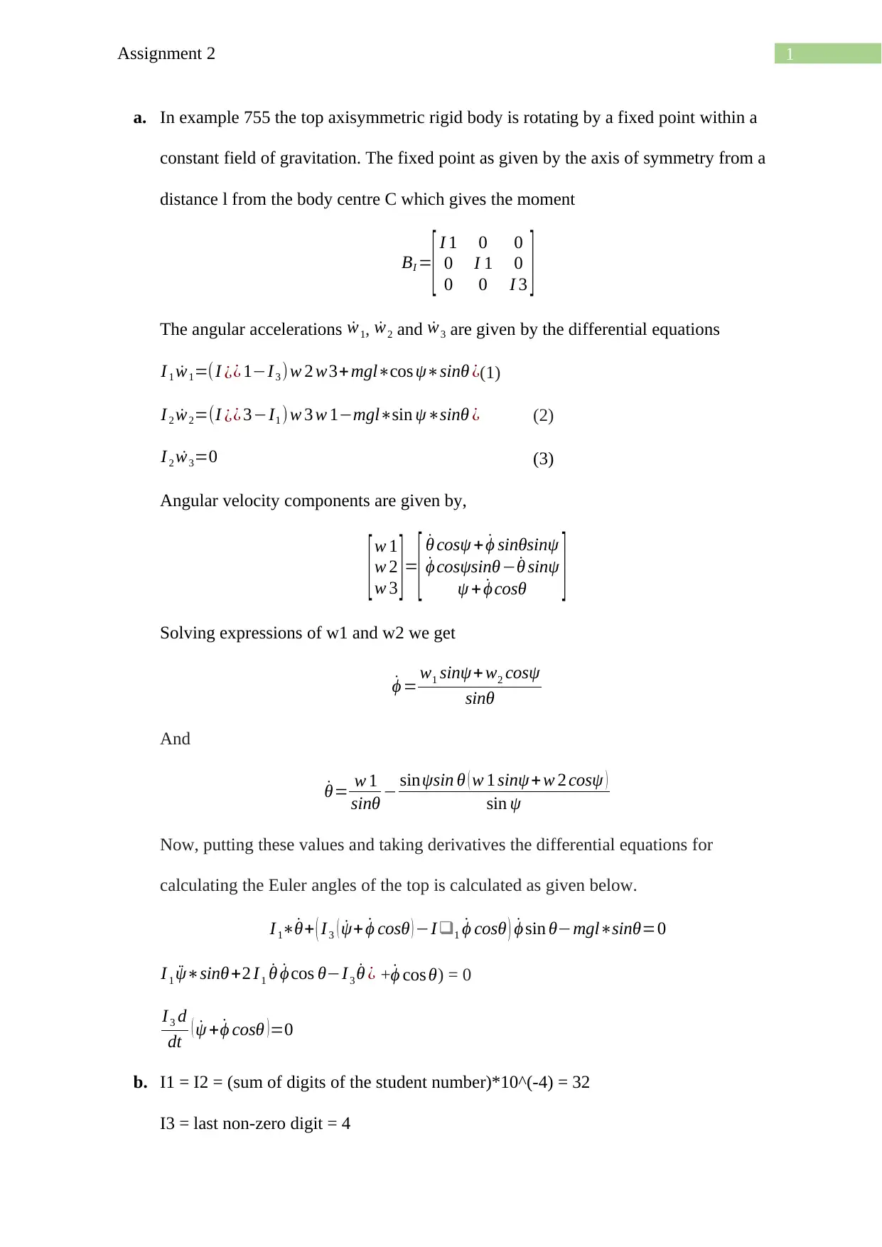
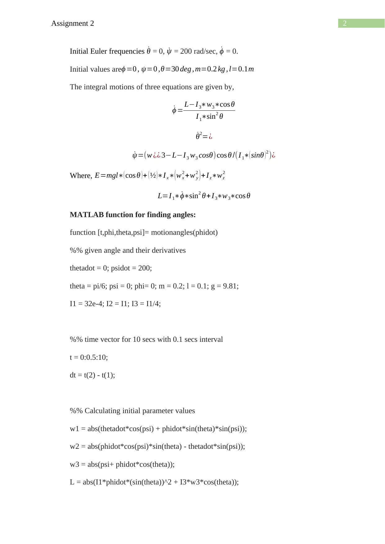
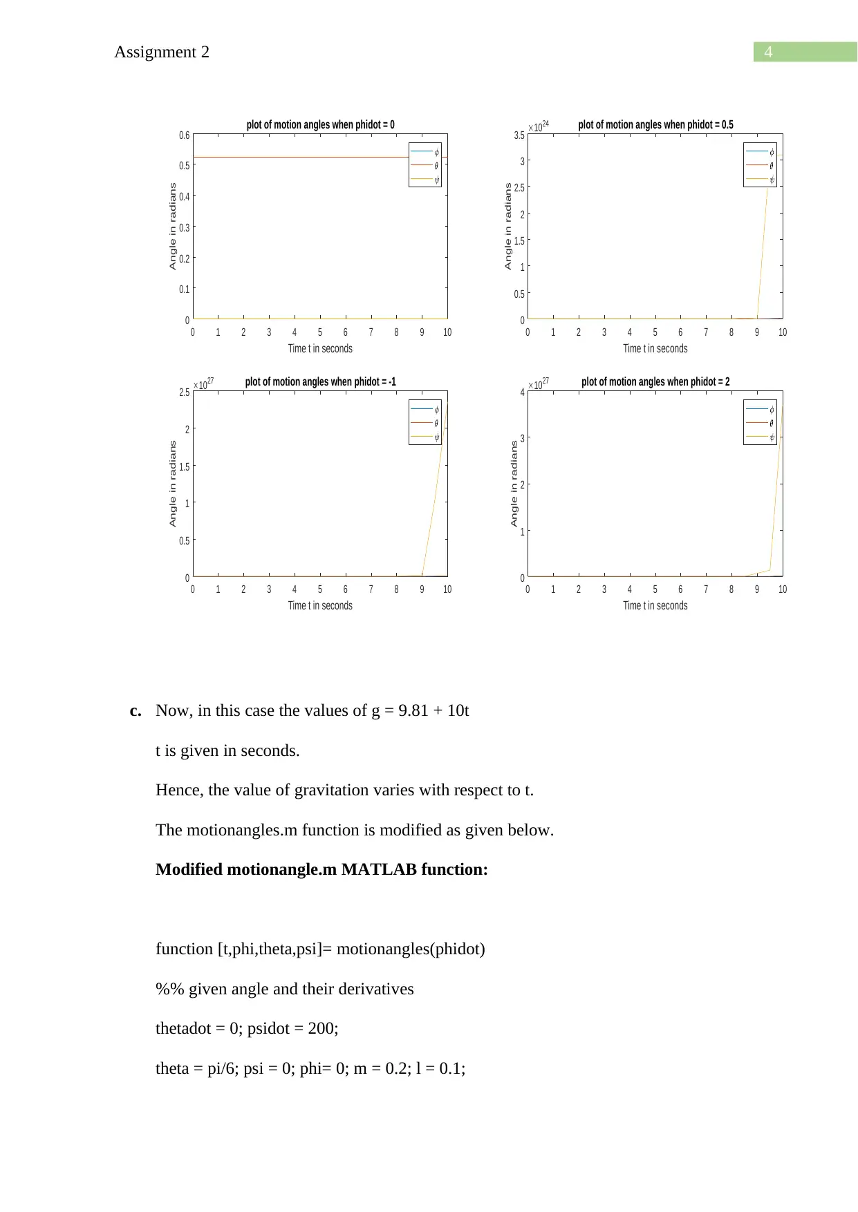
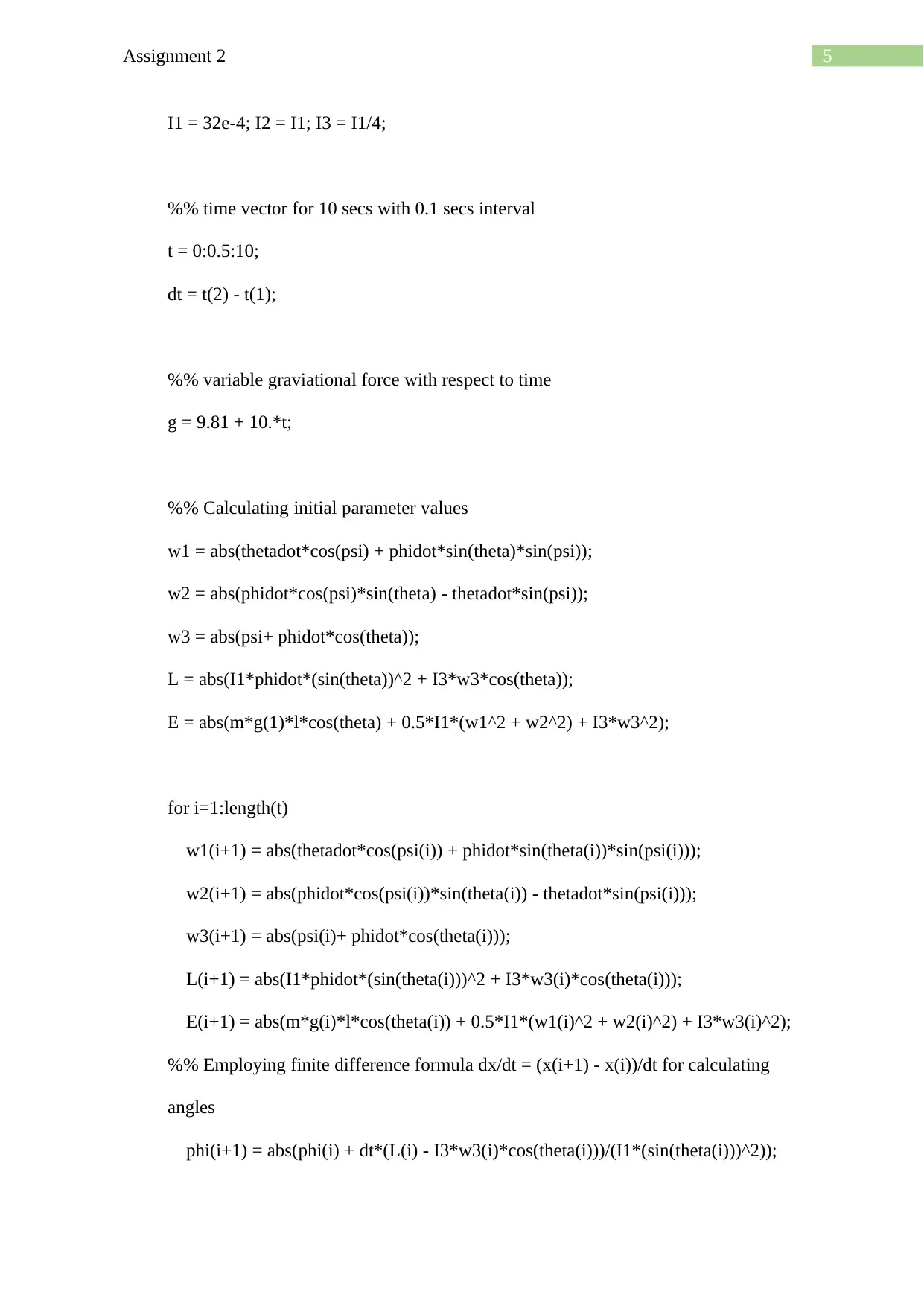
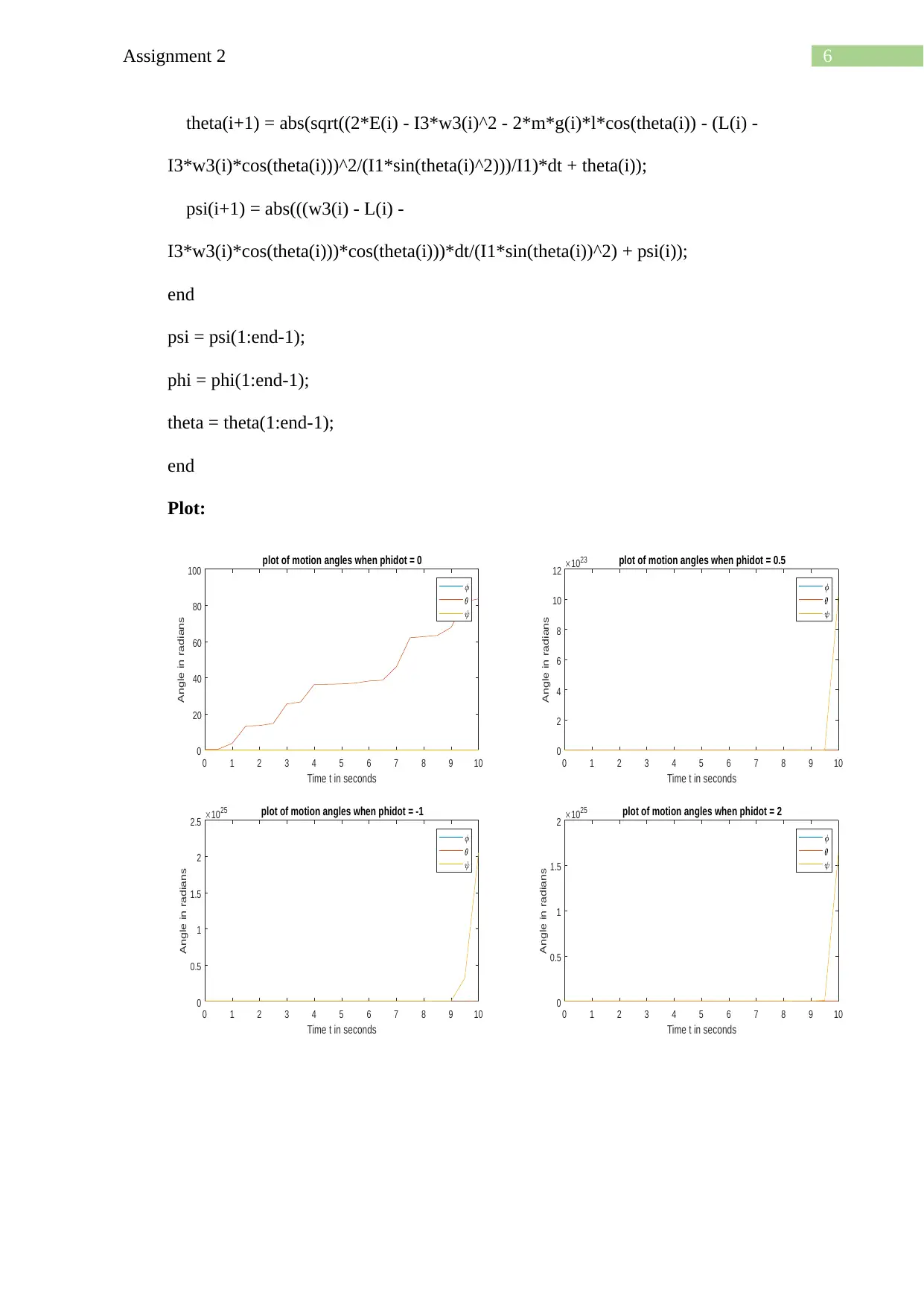
This document provides a complete solution to Assignment 2 on Top Dynamics, covering the analysis of a rotating axisymmetric rigid body under a constant gravitational field. The solution begins by redoing Example 755 from a textbook, deriving and proving the relevant differential equations and integrals of motion. It then proceeds to calculate and plot the possible motions of the top for various initial conditions, including a case with zero initial angular velocity. The assignment utilizes MATLAB to simulate the system, providing code for calculating Euler angles and plotting the results. Furthermore, the solution extends the analysis to a scenario where the gravitational acceleration varies with time, modifying the MATLAB code to accommodate this change and analyzing the resulting motion. The document includes detailed explanations, mathematical derivations, and MATLAB code snippets, making it a valuable resource for students studying mechanical engineering and dynamics.

Running head: Assignment 2
Assignment 2
Name of the Student
Name of the University
Author Note

1Assignment 2
a. In example 755 the top axisymmetric rigid body is rotating by a fixed point within a
constant field of gravitation. The fixed point as given by the axis of symmetry from a
distance l from the body centre C which gives the moment
BI =
[ I 1 0 0
0 I 1 0
0 0 I 3 ]
The angular accelerations ˙w1, ˙w2 and ˙w3 are given by the differential equations
I 1 ˙w1=(I ¿¿ 1−I 3 ) w 2 w3+ mgl∗cos ψ∗sinθ ¿(1)
I 2 ˙w2=(I ¿¿ 3−I1 ) w 3 w 1−mgl∗sin ψ∗sinθ ¿ (2)
I 2 ˙w3=0 (3)
Angular velocity components are given by,
[w 1
w 2
w 3 ]=
[ ˙θ cosψ + ˙ϕ sinθsinψ
˙ϕ cosψsinθ− ˙θ sinψ
ψ + ˙ϕ cosθ ]
Solving expressions of w1 and w2 we get
˙ϕ = w1 sinψ+ w2 cosψ
sinθ
And
˙θ= w 1
sinθ − sinψsin θ ( w 1 sinψ +w 2 cosψ )
sin ψ
Now, putting these values and taking derivatives the differential equations for
calculating the Euler angles of the top is calculated as given below.
I 1∗˙θ+ ( I3 ( ˙ψ+ ˙ϕ cosθ ) −I❑1 ˙ϕ cosθ ) ˙ϕ sin θ−mgl∗sinθ=0
I 1 ¨ψ∗sinθ+2 I 1 ˙θ ˙ϕ cos θ−I3 ˙θ ¿ + ˙ϕ cos θ) = 0
I 3 d
dt ( ˙ψ + ˙ϕ cosθ ) =0
b. I1 = I2 = (sum of digits of the student number)*10^(-4) = 32
I3 = last non-zero digit = 4

2Assignment 2
Initial Euler frequencies ˙θ = 0, ˙ψ = 200 rad/sec, ˙ϕ = 0.
Initial values areϕ =0 , ψ=0 ,θ=30 deg , m=0.2 kg , l=0.1m
The integral motions of three equations are given by,
˙ϕ = L−I 3∗w3∗cos θ
I 1∗sin2 θ
˙θ2=¿
˙ψ=(w ¿¿ 3−L−I 3 w3 cosθ)cos θ /(I 1∗( sinθ )2 )¿
Where, E=mgl∗( cos θ ) + ( ½ )∗I x∗( wx
2 +w y
2 ) + I z∗wz
2
L=I 1∗ ˙ϕ∗sin2 θ+I 3∗w3∗cos θ
MATLAB function for finding angles:
function [t,phi,theta,psi]= motionangles(phidot)
%% given angle and their derivatives
thetadot = 0; psidot = 200;
theta = pi/6; psi = 0; phi= 0; m = 0.2; l = 0.1; g = 9.81;
I1 = 32e-4; I2 = I1; I3 = I1/4;
%% time vector for 10 secs with 0.1 secs interval
t = 0:0.5:10;
dt = t(2) - t(1);
%% Calculating initial parameter values
w1 = abs(thetadot*cos(psi) + phidot*sin(theta)*sin(psi));
w2 = abs(phidot*cos(psi)*sin(theta) - thetadot*sin(psi));
w3 = abs(psi+ phidot*cos(theta));
L = abs(I1*phidot*(sin(theta))^2 + I3*w3*cos(theta));

3Assignment 2
E = abs(m*g*l*cos(theta) + 0.5*I1*(w1^2 + w2^2) + I3*w3^2);
for i=1:length(t)
w1(i+1) = abs(thetadot*cos(psi(i)) + phidot*sin(theta(i))*sin(psi(i)));
w2(i+1) = abs(phidot*cos(psi(i))*sin(theta(i)) - thetadot*sin(psi(i)));
w3(i+1) = abs(psi(i)+ phidot*cos(theta(i)));
L(i+1) = abs(I1*phidot*(sin(theta(i)))^2 + I3*w3(i)*cos(theta(i)));
E(i+1) = abs(m*g*l*cos(theta(i)) + 0.5*I1*(w1(i)^2 + w2(i)^2) + I3*w3(i)^2);
%% Employing finite difference formula dx/dt = (x(i+1) - x(i))/dt for calculating
angles
phi(i+1) = abs(phi(i) + dt*(L(i) - I3*w3(i)*cos(theta(i)))/(I1*(sin(theta(i)))^2));
theta(i+1) = abs(sqrt((2*E(i) - I3*w3(i)^2 - 2*m*g*l*cos(theta(i)) - (L(i) -
I3*w3(i)*cos(theta(i)))^2/(I1*sin(theta(i)^2)))/I1)*dt + theta(i));
psi(i+1) = abs(((w3(i) - L(i) -
I3*w3(i)*cos(theta(i)))*cos(theta(i)))*dt/(I1*sin(theta(i))^2) + psi(i));
end
psi = psi(1:end-1);
phi = phi(1:end-1);
theta = theta(1:end-1);
end
MATLAB code for plotting angles for different values of ˙ϕ:

4Assignment 2
0 1 2 3 4 5 6 7 8 9 10
Time t in seconds
0
0.1
0.2
0.3
0.4
0.5
0.6
Angle in radians
plot of motion angles when phidot = 0
0 1 2 3 4 5 6 7 8 9 10
Time t in seconds
0
0.5
1
1.5
2
2.5
3
3.5
Angle in radians
10 24 plot of motion angles when phidot = 0.5
0 1 2 3 4 5 6 7 8 9 10
Time t in seconds
0
0.5
1
1.5
2
2.5
Angle in radians
10 27 plot of motion angles when phidot = -1
0 1 2 3 4 5 6 7 8 9 10
Time t in seconds
0
1
2
3
4
Angle in radians
10 27 plot of motion angles when phidot = 2
c. Now, in this case the values of g = 9.81 + 10t
t is given in seconds.
Hence, the value of gravitation varies with respect to t.
The motionangles.m function is modified as given below.
Modified motionangle.m MATLAB function:
function [t,phi,theta,psi]= motionangles(phidot)
%% given angle and their derivatives
thetadot = 0; psidot = 200;
theta = pi/6; psi = 0; phi= 0; m = 0.2; l = 0.1;

5Assignment 2
I1 = 32e-4; I2 = I1; I3 = I1/4;
%% time vector for 10 secs with 0.1 secs interval
t = 0:0.5:10;
dt = t(2) - t(1);
%% variable graviational force with respect to time
g = 9.81 + 10.*t;
%% Calculating initial parameter values
w1 = abs(thetadot*cos(psi) + phidot*sin(theta)*sin(psi));
w2 = abs(phidot*cos(psi)*sin(theta) - thetadot*sin(psi));
w3 = abs(psi+ phidot*cos(theta));
L = abs(I1*phidot*(sin(theta))^2 + I3*w3*cos(theta));
E = abs(m*g(1)*l*cos(theta) + 0.5*I1*(w1^2 + w2^2) + I3*w3^2);
for i=1:length(t)
w1(i+1) = abs(thetadot*cos(psi(i)) + phidot*sin(theta(i))*sin(psi(i)));
w2(i+1) = abs(phidot*cos(psi(i))*sin(theta(i)) - thetadot*sin(psi(i)));
w3(i+1) = abs(psi(i)+ phidot*cos(theta(i)));
L(i+1) = abs(I1*phidot*(sin(theta(i)))^2 + I3*w3(i)*cos(theta(i)));
E(i+1) = abs(m*g(i)*l*cos(theta(i)) + 0.5*I1*(w1(i)^2 + w2(i)^2) + I3*w3(i)^2);
%% Employing finite difference formula dx/dt = (x(i+1) - x(i))/dt for calculating
angles
phi(i+1) = abs(phi(i) + dt*(L(i) - I3*w3(i)*cos(theta(i)))/(I1*(sin(theta(i)))^2));

6Assignment 2
theta(i+1) = abs(sqrt((2*E(i) - I3*w3(i)^2 - 2*m*g(i)*l*cos(theta(i)) - (L(i) -
I3*w3(i)*cos(theta(i)))^2/(I1*sin(theta(i)^2)))/I1)*dt + theta(i));
psi(i+1) = abs(((w3(i) - L(i) -
I3*w3(i)*cos(theta(i)))*cos(theta(i)))*dt/(I1*sin(theta(i))^2) + psi(i));
end
psi = psi(1:end-1);
phi = phi(1:end-1);
theta = theta(1:end-1);
end
Plot:
0 1 2 3 4 5 6 7 8 9 10
Time t in seconds
0
20
40
60
80
100
Angle in radians
plot of motion angles when phidot = 0
0 1 2 3 4 5 6 7 8 9 10
Time t in seconds
0
2
4
6
8
10
12
Angle in radians
10 23 plot of motion angles when phidot = 0.5
0 1 2 3 4 5 6 7 8 9 10
Time t in seconds
0
0.5
1
1.5
2
2.5
Angle in radians
10 25 plot of motion angles when phidot = -1
0 1 2 3 4 5 6 7 8 9 10
Time t in seconds
0
0.5
1
1.5
2
Angle in radians
10 25 plot of motion angles when phidot = 2

7Assignment 2
Hence, it can be seen from the above plots that with variable gravitational force the angles
theta is changing with time even if the change of phi is zero, however, other angles are
constant.