University Power System Analysis and Control Assignment 1

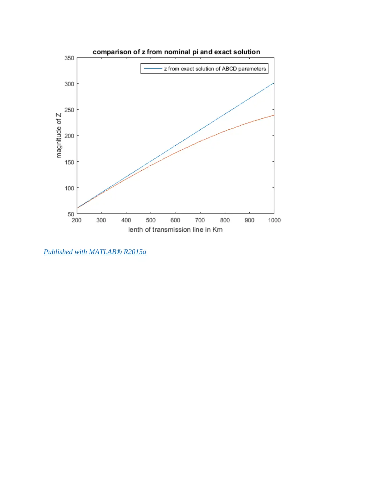
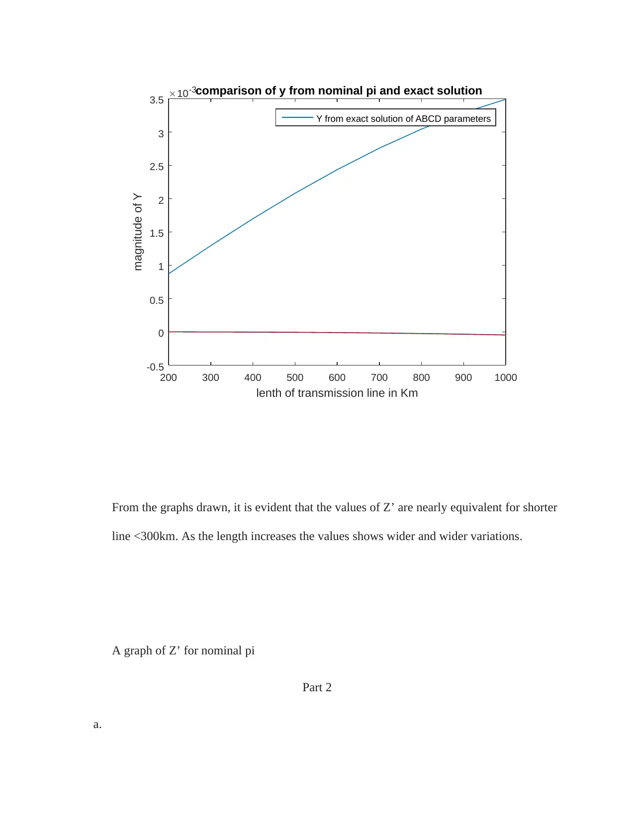
This document presents a comprehensive solution to a Power System Analysis assignment, focusing on key concepts such as transmission line parameters, modeling, and power transfer limits. The solution begins by analyzing the series impedance, shunt admittance, propagation constant, and characteristic impedance of a transmission line, comparing the results obtained from exact and nominal pi models. It further explores power transfer calculations, determining maximum real power, and analyzing the impact of line length on power delivery. The assignment also delves into the effects of series compensation and voltage regulation, comparing the performance of transmission lines at different voltage levels. The solution includes detailed calculations, MATLAB code, and graphical representations to illustrate the concepts and findings. The assignment covers topics like ABCD parameters, characteristic impedance, and the impact of compensation on power transfer capabilities. The solution also analyzes the sending end voltage and regulation, comparing the performance at different voltage levels.

Part 1
a. From the obtained dataset, the series impedance z=¿0.0166+j0.301 and the shunt
admittance y= j 4.4 ×10−6
i. The propagation constant
γ= √zy
From the obtained dataset, the series impedance z=¿0.0166+j0.301 and the shunt
admittance y= j 4.4 ×10−6
γ= √( ( 0.0166+ j0.301 ) ׿ ( j 4.4 × 10−6 ) )¿
γ= ( √1.3264 10−6 )< 176.84
2
3.17554 ×10−5 +1.1513i ×10−3
ii. The characteristic impedance zc
zc= √ z
y
Substituting the variables
zc= √ 0.0166+ j 0.301
j 4.4 ×10−6
zc= √68513.034< −3.1566
2
261.651−7.2093 i

iii. The exact ABCD parameters
A=D=cosh γl
B=zc sinh γl
C= 1
zc
sinh γl
But l=292 km
γ l= ( 3.17554 ×10−5 +1.1513i ×10−3 ) × 292
9.27258 ×10−3+3.3706i ×10−1
cosh γl= αejβ +αe− jβ
2 = ( 9.27258× 10−3 ) < ( 3.3706i ×10−1 ) + ( 9.27258 ×10−3 ) < ( 3.3706i ×10−1 )
2
A=D=9.4407 × 10−1 <1.8544 ×10−1
sinh γ = αe jβl−αe− jβ
2
( 9.27258 ×10−3 ) < ( 3.3706 i ×10−1 ) − ( 9.27258× 10−3 ) < ( 3.3706 i ×10−1 )
2
B= ( ( 9.27258 ×10−3 ) < ( 3.3706i ×10−1 ) − ( 9.27258 ×10−3 ) < ( 3.3706 i× 10−1 )
2 ) ×261.651−7.2093i
B=8.6378 × 101< 8.6903× 101 ohms

C=( ( 9.27258 ×10−3 ) < ( 3.3706 i× 10−1 )− ( 9.27258× 10−3 ) < ( 3.3706i ×10−1 )
2
261.651−7.2093 i )
1.2608 ×10−3 <9.0060× 101 Siemens
iv. The exact nominal pi Z’ Y’ parameters
ˇz=Z= ( 0.0166+ j 0.301 )
ˇZ=86.378<86.903
ˇy= y (1+ yz
4 )
ˇy=( j 4.4 ×10−6
(1+ ( j 4.4 ×10−6 ) ( 0.0166+ j 0.301 )
4 ))× 292
ˇy=6.7912×10−7 +i1.2970 ×10−3
b. Comparison between Z’ and Y’ for the exact and nominal pi
In accurate solutions of the parameters,
Z’=B
Y’=C

x=[200 300 400 500 600 700 800 900 1000];
z=0.0166+0.301i;
y=0.0000044i;
l=0.0000317554+0.0011513i;
Zc=261.651-7.2093i;
Zpi=abs(Z*x)
Zex=abs((sinh(x*l))*Zc)
plot(x,Zpi)
hold on
plot(x,Zex)
legend('z from nominal pi')
legend('z from exact solution of ABCD parameters')
title (' comparison of z from nominal pi and exact solution')
xlabel('lenth of transmission line in Km')
ylabel('magnitude of Z')
Zpi =
Columns 1 through 7
60.2915 90.4372 120.5830 150.7287 180.8744 211.0202 241.1659

Columns 8 through 9
271.3117 301.4574
Zex =
Columns 1 through 7
59.7626 88.6542 116.3730 142.5523 166.8458 188.9323 208.5198
Columns 8 through 9
225.3497 239.1995

Published with MATLAB® R2015a

lenth of transmission line in Km
200 300 400 500 600 700 800 900 1000
magnitude of Y
10-3
-0.5
0
0.5
1
1.5
2
2.5
3
3.5 comparison of y from nominal pi and exact solution
Y from exact solution of ABCD parameters
From the graphs drawn, it is evident that the values of Z’ are nearly equivalent for shorter
line <300km. As the length increases the values shows wider and wider variations.
A graph of Z’ for nominal pi
Part 2
a.

i.
surge impedance=Real ( zc ) =261.651
SIL ( MW ) = k V L−L
2
surge impedance = 7502
261.651 =2148.9974 MW
ii. From the power transfer formulae below, we have
PR= V R V S
B cos ( θB−δ ) − A V R
2
B cos ( θB −θA )
QR= V R V S
B sin ( θB−δ )− A V R
2
B sin ( θB−θ A )
B=86.378<86.903
A=0.9441<0.18544
For maximum real power, the reactive power has to be zero
Hence
QR= V R V S
B sin ( θB−δ )− A V R
2
B sin (θB−θ A )=0
But V R ¿ V S
Hence
1
86.378 sin ( θB−δ ) =¿ 0.9441
86.378 sin ( 86.903−0.18544 ) ¿

sin ( θB−δ ) =¿ 0.94255 ¿
( θB−δ ) =70.4845
Substituting the value of ( θB−δ ) in the real part of the equation, we get
PR= 750× 750
86.378 cos 70.4845− 0.9441×7502
86.378 cos ( 86.7176 )
1823.415 MW
As a percentage of SIL,
1823.415 MW
2148.9974 MW × 100=84.84955%
b. When the transmission line is operated at 500kV,
V R ¿ V S=500 kV
SIL ( MW )= k V L−L
2
surge impedance = 5002
261.651 =955.4712 MW
¿ 955.4712 MW
Maximum real power loading
Since
V R ¿ V S
From part b,

1
86.378 sin ( θB−δ ) =¿ 0.9441
86.378 sin ( 86.903−0.18544 ) ¿
sin ( θB−δ ) =¿ 0.94255 ¿
( θB−δ ) =70.4845
Substituting, we obtain
PR= 500× 500
86.378 cos 70.4845− 0.9441×5002
86.378 cos ( 86.7176 )
810.4065 MW
Part 3
a.
i.
PR= V R V S
B cos ( θB−δ ) − A V R
2
B cos ( θB −θA )
QR= V R V S
B sin ( θB−δ )− A V R
2
B sin ( θB−θ A )
V S =Vbase ×Vspu=1.02× 750=765 kv
V R=Vbase × Vspu=0.98 ×750=735 kv
δ =δmax=36

PR= 765× 735
86.378 cos (86.903−36)− 0.9441×7352
86.378 cos ( 86.7176 )
3768.9270 MW
SIL ( MW ) = k V L−L
2
surge impedance = 7502
261.651 =2148.9974 MW
As a percentage of SIL,
3768.9270
2148.9974 MW × 100=175.3381 %
b.
Vbase=500 kv
V S =Vbase ×Vspu=1.02× 500=510 kv
V R=Vbase × Vspu=0.98 ×500=490 kv
From part a, we have
PR= V R V S
B cos ( θB−δ ) − A V R
2
B cos ( θB −θA )
QR= V R V S
B sin ( θB−δ )− A V R
2
B sin ( θB−θ A )
PR= 510× 490
86.378 cos(86.903−36)− 0.9441 ×4902
86.378 cos ( 86.7176 )
Practical loadability 1674.2310 MW

Part 4
i.
V s =AV R + B I R
V R=Vbase × VRpu=750× 0.96=729 kv
V R=720 KV < 0
I R =1.90 KA <0
A=0.9441<0.18544
B=86.378<86.903
Substituting the variables in the equation, we get
V s =((0.9441<0.18544)720<0)+( ( 86.378< 86.903 ) (1.90< 0 ) )
708.3593<13.5595 KV
ii. Under no load,
I R =0
V s =AV R
V R=¿ 708.3593 <13.5595
(0.9441<0.18544) ¿
V NL=751.8252<13.3387
iii.

%Regulation=
|V NL|−|V FL|
|V FL| ×100
%Regulation=751.8252−720
720 ×100
4.4202 %
Part 5
a.
i. From the problem description
ˇz=86.378< 86.903
Y '=G' + j (1− eshunt
100 )B '
ˇy=6.7912×10−7 +i1.2970 ×10−3
Y ' =6.7912 ×10−7+ j ( 1− 75
100 ) 1.2970 ×10−3
Y ' =6.7912 ×10−7+ j3.2425 × 10−4
From the new values of Y’ and Z’, we have
From part 1,
The characteristic impedance zc
zc= √ z
y
Substituting the variables
zc= √ 86.378<86.903
6.7912 ×10−7+ j 3.2425× 10−4

zc= √266392.63< −2.9769
2
γ= √(86.378<86.903 ׿ ( 6.7912× 10−7 + j3.2425 ×10−4 ) )¿
γ= √0.028001< 176.78
2 =4.7014 × 10−3 +0.1673 i
i. The exact ABCD parameters
A=D=cosh γl
B=zc sinh γl
C= 1
zc
sinh γl
But l=292
cosh γl= αejβ +αe− jβ
2 = ( 4.7014 ×10−3 )< ( 0.1673 ) + ( 4.7014 ×10−3 )< ( 0.1673 )
2
A=D=0.98602<4.567 ×10−2
sinh γ = αe jβl−αe− jβ
2

( 4.7014 × 10−3 ) < ( 0.1673 )− ( 4.7014 ×10−3 ) < ( 0.1673 )
2
B= sinh γ
zc
( 4.7014 × 10−3 ) < ( 0.1673 )− ( 4.7014 ×10−3 ) < ( 0.1673 )
2 ÷ zc= √266392.63<−2.9769
2
B=86.378<86.903
ii.
V s =AV R + B I R
V R=Vbase × VRpu=750× 0.96=720 kv
V R=720 KV < 0
I R =1.90 KA <0
A=0.98602<4.567 ×10−2
B=86.378<86.903
Substituting the variables, we get
V s =((0.98602<4.567 × 10−2 )720<0)+( ( 86.378<86.903 ) ( 1.90<0 ) )
737.3715<12.8861
Sending end voltage 737.3715 kV
Power angle=12.8861degrees

iii.
Sending end voltage from part 4 = 708.3593<13.5595 KV
A=0.98602<4.567 ×10−2
I R =0
V s =AV R
V R=¿ 708.3593<13.5595
0.98602<4.567 ×10−2 ¿
V NL=718.402<13.51383
iv.
I R =0
V s =AV R
%Regulation=
|V NL|−|V FL|
|V FL| ×100
V R=¿ 737.3715<12.8861
0.98602 <4.567 ×10−2 =747.8261 <0.2740¿
%Regulation=747.8261−720
720 ×100=0.03865 %

v.
I R =0
V s =AV R
V R= V s
A = 708.3593<13.5595
0.98602<4.567 ×10−2 =718.403<13.51333
%Regulation=718.402−720
720 ×100=0.22194 %
vi.
b.
V s =AV R + B I R
V R=Vbase × VRpu=750× 0.96=720 kv
V R=490 KV <0
I R =1.90 KA <0

A=0.98602<4.567 ×10−2
B=86.378<86.903
Substituting the variables, we get
V s =((0.98602<4.567 × 10−2 ) 490<0)+( ( 86.378<86.903 ) ( 1.90< 0 ) )
Sending end voltage 518.7225 kV
Power angle=18.46200 degrees
Sending end voltage from part 4 =518.7225 kV <18.46200 KV
A=0.98602<4.567 ×10−2
I R =0
V s =AV R
V R=¿ 518.7225 kV <18.46200 KV
0.98602< 4.567× 10−2 ¿
V NL=526.066<18.41633
%Regulation=526.066−490
490 ×100=7.3604 %
Regulation is worse at 500kV compared to 750kV

Part 6
a.
i.
Zcap=− j 1
2 ´X × eseries
100
But Z=R+jX
ˇZ=86.378<86.903=4.6667+ j 86.2518
´X =86.2518
Zcap=− j 1
2 ´×86.2518 × 30
100 =− j12.93777
ii.
( Aeq Beq
Ceq Deq
)=(1 Zcap
0 1 ) ( A B
C D ) (1 Zcap
0 1 )
(1 − j12.93777
0 1 )× (0.94407<0.18544 86.378< 86.903
0.0012608<90.06 0.94407<0.18544 )× (1 − j 12.93777
0 1 )
0.986019<0.04567 86.378<86.903
0.0012610<90.06 0.98602<0.04567

A=0.986019<0.04567
B=86.378< 86.90
iii.
PR= V R ,com V S com
Beq cos ( θBeq −δ )− Aeq V Rcom
2
Beq cos ( θB , eq−θ A , eq )
QR= V R ,com V S com
Beq sin ( θBeq−δ ) − Aeq V Rcom
2
Beq sin ( θB ,eq −θA , eq ) ..1
For maximum loading, QR=0
QR= V R ,com V S com
Beq sin ( θBeq−δ ) − Aeq V Rcom
2
Beq sin ( θB ,eq −θA , eq ) =0. .2
since
|V R , com|=|V s ,com|=V rated
0.986019
86.378 sin ( 86.90−0.04567 ) = 1
86.378 sin ( θBeq −δ )
hence ( θBeq −δ )=79.90985
hence
PR= 750× 750
86.378 cos 79.90985− 0.986019× 7502
86.378 cos ( 86.85433 )
788.5468 MW
iv.
From part 2 ii, the maximum real power value

PR=1823.415 MW
From part 6 iii, we have
PR=788.5468 MW
The difference =1823.415 MW −788.5468 MW =1034.8682 MW
As per percentage of the difference in maximum power of SIL, we have
1034.8682 MW
2148.9974 MW × 100=48.1559 %
v.
PR= V R V S
B cos ( θB−δ ) − A V R
2
B cos ( θB −θA )
QR= V R V S
B sin ( θB−δ )− A V R
2
B sin (θB−θ A )
V S =Vbase ×Vspu=1.02× 750=765 kv
V R=Vbase × Vspu=0.98 ×750=735 kv
δ=δmax=36
PR= 765× 735
86.378 cos (86.90−36)− 0.986019× 7352
86.378 cos ( 86.85433 )
PR=3766.966194 MW
vi.

The difference between the practical maximum real power delivery values of
the uncompensated transmission line of part 3a and the compensated
transmission
From part 3a,
PR=3768.9270 MW
From 6 v,
PR=3766.966194 MW
The difference = PR=3766.966194 MW −3766.966194 MW =1.960806 MW
Expressed as percentage of SIL,
1.960806 MW
2148.9974 MW × 100=0.0912%
b.
From par 6 a v, we have the receiving end power relations as
PR= V R V S
B cos ( θB−δ ) − A V R
2
B cos ( θB −θA )
QR= V R V S
B sin ( θB−δ )− A V R
2
B sin (θB−θ A )
V S =Vbase ×Vspu=1.02× 500=510 kv
V R=Vbase × Vspu=0.98 ×500=490 kv
δ=δmax=36