Travelling Salesperson Problem (TSP) Model Analysis and Solution

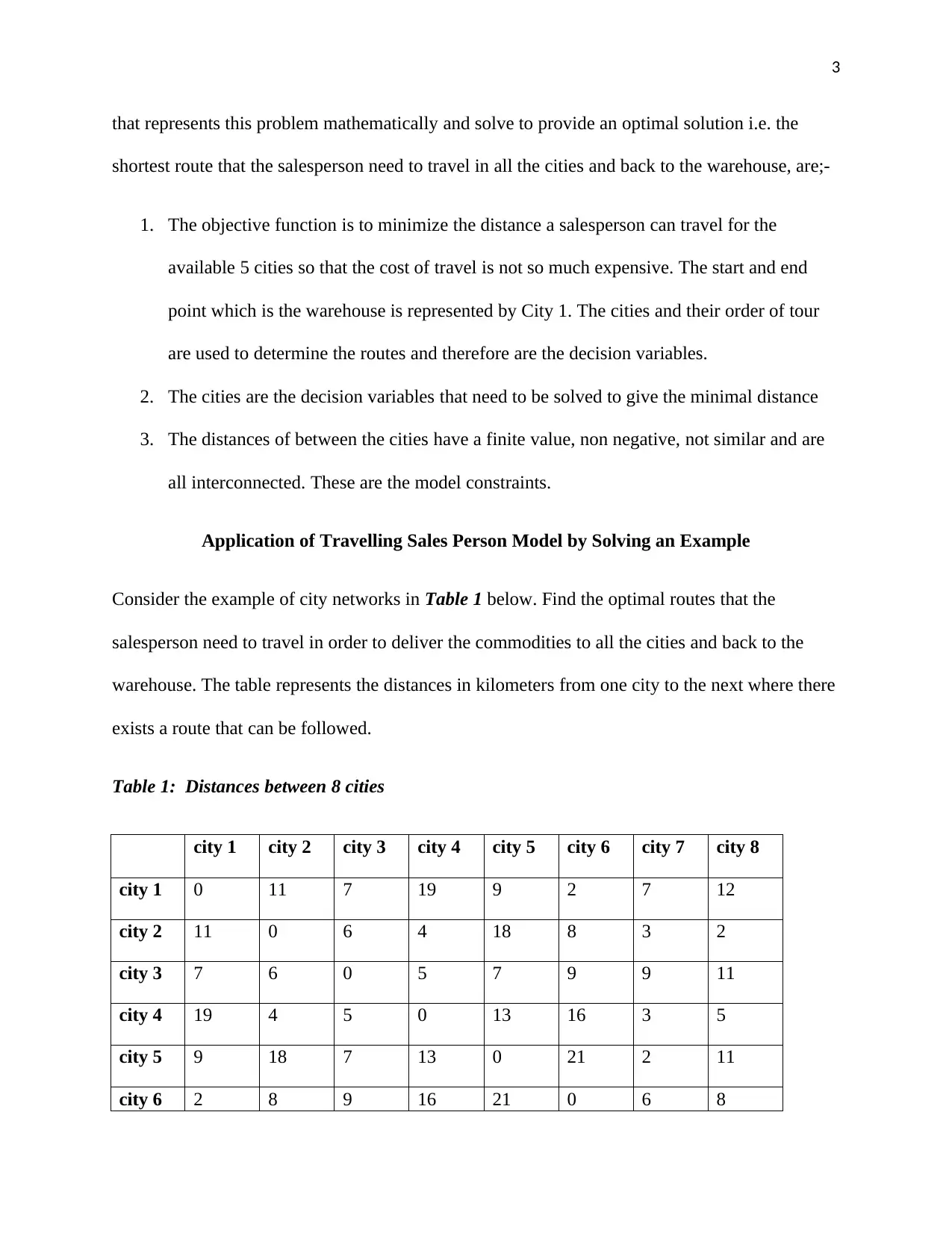
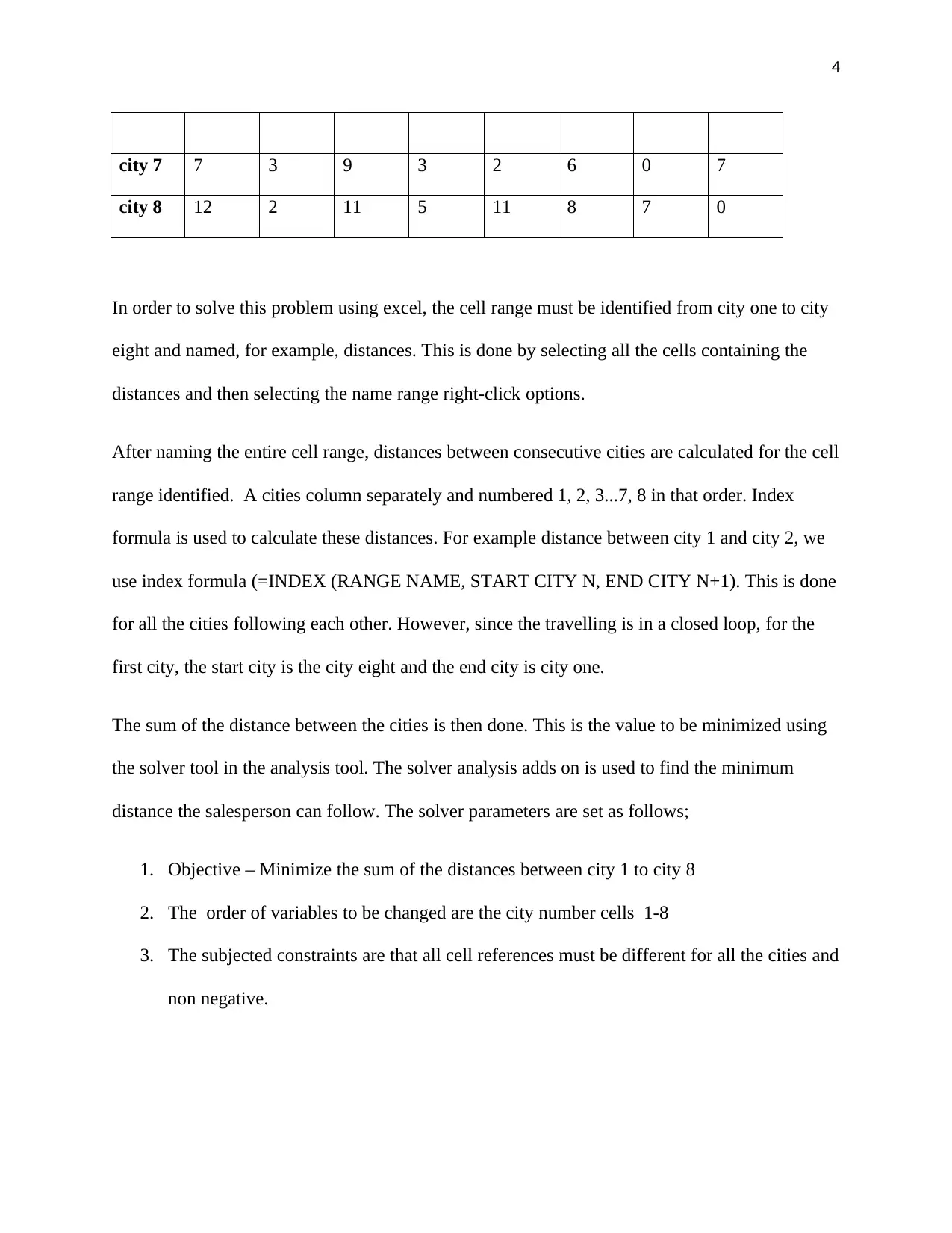
This project analyzes the Travelling Salesperson Problem (TSP), a crucial model in operations research used to determine the shortest route for a salesperson visiting multiple locations. The document provides a detailed background of the TSP, explaining its objective of minimizing travel costs and maximizing efficiency. It presents the typical mathematical model, including the objective function, decision variables (cities and their order), and constraints (distances between cities). The project includes a practical example with eight cities, demonstrating how to solve the TSP using Excel's Solver tool. The solution reveals the optimal route, minimizing the total distance traveled. Additionally, a literature review explores various applications of the TSP, such as route optimization in supply chains, robotic drilling, and real-time traffic analysis in Google Maps. The document concludes by emphasizing the TSP's suitability for analyzing supply chains, highlighting the use of evolutionary algorithms to find optimal paths, and acknowledging the advancements in technologies like Google Maps that simplify route planning. The project also includes a list of references used to support the analysis.

1
TRAVELLING SALES PERSON MODEL (TSP) (ANALYSIS
By
Name
Professor’s Name
Course Number
College/University Name
Street
Date

2
Travelling Sales Person Model (TSP)
Background Information
TSP model is a operations research analysis of determining the shortest routes a delivery sales
person can use to supply his/her commodities to the customers located at different locations with
interconnecting routes (Matai, Singh, & Mittal, 2010). By elimination, this model provides an
interconnected order of routes that the sales person uses so that the shortest and most economic
route is used from the distribution store, across to all customers and then back to the store.
The shortest route is the optimal solution for the distributor that will enable him/her to maximize
the output of goods delivered to customers while minimizing the cost of travelling to those
customers.
Typical Mathematical Model of TSP
The mathematical model of Traveling Salesperson Problem is represented by a list a points
possibly cities called nodes. These are the locations where the supplies are to be made to be
made. i and j notations are used to assign the departure and destinations for the given nodes
where i is the departure point at a given city and j is the destination point at the next city. In
addition, the distances or the time taken to travel from one point to another must also be known
for this model to work out.
To formulate a complete operations research model, we first need to identify three basic aspects
of the problem in question i.e. the objective function, the decision variable and the constraints of
the decision variables. For example; if we have 5 cities that a salesperson need to supply his
products from the warehouse (city 1), the aspects that must be considered to develop a model

3
that represents this problem mathematically and solve to provide an optimal solution i.e. the
shortest route that the salesperson need to travel in all the cities and back to the warehouse, are;-
1. The objective function is to minimize the distance a salesperson can travel for the
available 5 cities so that the cost of travel is not so much expensive. The start and end
point which is the warehouse is represented by City 1. The cities and their order of tour
are used to determine the routes and therefore are the decision variables.
2. The cities are the decision variables that need to be solved to give the minimal distance
3. The distances of between the cities have a finite value, non negative, not similar and are
all interconnected. These are the model constraints.
Application of Travelling Sales Person Model by Solving an Example
Consider the example of city networks in Table 1 below. Find the optimal routes that the
salesperson need to travel in order to deliver the commodities to all the cities and back to the
warehouse. The table represents the distances in kilometers from one city to the next where there
exists a route that can be followed.
Table 1: Distances between 8 cities
city 1 city 2 city 3 city 4 city 5 city 6 city 7 city 8
city 1 0 11 7 19 9 2 7 12
city 2 11 0 6 4 18 8 3 2
city 3 7 6 0 5 7 9 9 11
city 4 19 4 5 0 13 16 3 5
city 5 9 18 7 13 0 21 2 11
city 6 2 8 9 16 21 0 6 8

4
city 7 7 3 9 3 2 6 0 7
city 8 12 2 11 5 11 8 7 0
In order to solve this problem using excel, the cell range must be identified from city one to city
eight and named, for example, distances. This is done by selecting all the cells containing the
distances and then selecting the name range right-click options.
After naming the entire cell range, distances between consecutive cities are calculated for the cell
range identified. A cities column separately and numbered 1, 2, 3...7, 8 in that order. Index
formula is used to calculate these distances. For example distance between city 1 and city 2, we
use index formula (=INDEX (RANGE NAME, START CITY N, END CITY N+1). This is done
for all the cities following each other. However, since the travelling is in a closed loop, for the
first city, the start city is the city eight and the end city is city one.
The sum of the distance between the cities is then done. This is the value to be minimized using
the solver tool in the analysis tool. The solver analysis adds on is used to find the minimum
distance the salesperson can follow. The solver parameters are set as follows;
1. Objective – Minimize the sum of the distances between city 1 to city 8
2. The order of variables to be changed are the city number cells 1-8
3. The subjected constraints are that all cell references must be different for all the cities and
non negative.

5
N/B. Evolutionary engine is used to terminate the process when the most optimal solution is
achieved. This is the algorithm that the solver uses to run simultaneous available options of
complete loop touching all the cities and ensuring none is repeated.
The analysis is then done by clicking on the solve button. Excel runs this process and provides an
optimal solution of the most suitable shortest and economic route.
Shortest route excel solution
Table 2: Optimal excel solution
City Distance
3 7
5 7
7 2
4 3
2 4
8 2
6 8
1 2
Total distance 35
From the solution in Table 2 , it is evident that the most viable route the salesperson can follow
is through routes 3 → 5 → 7 → 4→ 2→ 8→6 → 1 and then back to 3. This gives a total distance
of 35kilometeres for the entire travelling to deliver commodities.

6
The table shows that the delivery should start at city 3 and end in city 1 then back to city 3.
However since it is a closed loop, the start and end doesn’t matter. The salesperson location can
be anywhere among the eight cities. Rearranging it and taking city 1 as the warehouse location of
the salesperson, the routes he/she should follow is 1→3 → 5 → 7 → 4→ 2→ 8→6 → 1

7
Literature review of Travelling Sales Person Model
Focus is given on the travelling salesperson problem in minimizing the cost of travel to different
regions he/she needs to sell the goods by choosing shortest route to each of the regions by the use
the dynamic programming algorithm to solve this problem for a network of four towns.
According to Obioma, Ogwude, and Galadima (2014) findings, there are no great complications
in using this model to find shortest route though there is a need for a bit realistic models for
routing problems with advanced and efficient computing algorithms involving delivery of
commodities to different towns of limited numbers.
Grötschel, Jünger, and Reinelt (1991) attempt to apply the Travelling Sales person Problem in
the drilling of circuit boards for electronic purposes using robots. For all connections of
conductors to one another, holes have to be drilled in the circuit board. Different conductors
require different holes of different sizes. This necessitates the need to drilled using different drill
equipments. The robot thus has to therefore change the drills occasionally during the drilling
period. A lot of time is wasted during these changes. However, TSP can be used to find the short
path. The cities represent the positions to be drilled. The time taken to move from one hole to the
next is the ‘distance’ between two different drills positions.
The travelling salesperson problem has also been used in Google Maps technology to develop an
algorithm that analyses the available routes with the knowledge of intensity of the traffic.
According to Erol and Bulut (2017), for example if you want to travel from point A to point B,
this algorithm analyses the available routes and the intensity of traffic using several methods like
branch and bound algorithm and gives the shortest according to duration and distance. This
feature now exists in the Google Maps application.

8
According to Ratliff and Rosenthal (1983), travelling salesperson can be used to solve the
problem of material handling in a warehouse efficiently. For example if you have several items
in a warehouse that is rectangular in shape and contain crossovers both ends of the aisles, the
supply of these items may be efficient if travelling salesperson problem operation research model
is used. An evolutionary algorithm can be generated to minimize the time taken to pick an order
within the warehouse from one point to another.
Rakke et al. (2012) provides an in depth illustration of how one can apply the Travelling
salesperson problem to do routing of the marine ships under draft limit constraints in the ports.
Draft limit represents the distance top surface of the water on the ship and the ship’s bottom and
is affected by the loads being carried on the ship. This greatly affects the docking of a ship at a
particular port. An algorithm therefore has to be determined to find the best possible sequence of
routes the ship has to travel while offloading goods so as not to be constrained by the waterline at
some of the ports (Rakke et al., 2012). They find out that introducing limits hardens the solution
process. In addition, their findings indicate that the proposed inequalities and bounds greatly
reduce the time of finding a solution and number nodes.
Most of these articles attempt to find the shortest route of a supply chain in different sectors such
as travelling to a given destination, delivery of commodities, and robotic works in a
manufacturing plant e.tc. Even though different algorithms are used, the optimal solution is
obtained isn’t so much different. The error is too small. Some of the algorithms used in finding
optimal solution assume that the paths are linear while others assume non-linear paths (Rakke et
al., 2012). For example the supply of commodities algorithm to several towns assumed a non
liner path while the pick and delivery of items in a warehouse assume a linear path in a number
of aisles. Some also use a branch and bound algorithm.

9
Travelling salesperson problem is considered the most suitable way of analyzing the supply
chains of commodities either within a warehouse, to customers, or in integrated systems where
distance and duration is a factor to be considered.
Evolutionary algorithm is used to easily provide the shortest path that can be followed with all
constraints considered. However, unlike multiple travelling salesperson problems, this model
only provides for solution of one path and pass in the entire system. The supply chain is
considered to be only once to each destination (Matai, Singh, & Mittal, 2010). Despite the
number of cities, the evolutionary algorithm solver incorporated in Microsoft excel can be used
to obtain the most suitable path though it takes a lot of time to do the analysis. This has been
made easier by the Google maps application which uses the GPS satellite system to measure
distances between cities and come up with the best route easily and within a short time. Dynamic
programming approach also has a drawback on the number of destinations to be considered. It
cannot handle a large number.
Summary of findings
In conclusion, travelling salesperson problem model is the most appropriate method of
determining the shortest route of a supply chain as it has several application areas and has several
algorithms that can be used but it does apply only in single path supplies where the supplier
doesn’t need to travel to a destination more than once.

10
References
Erol, M.H. and Bulut, F., 2017, April. Real-time application of travelling salesman problem
using Google Maps API. In 2017 Electric Electronics, Computer Science, Biomedical
Engineerings' Meeting (EBBT) (pp. 1-5). IEEE. doi:10.1109/EBBT.2017.7956764
Grötschel, M., Jünger, M. and Reinelt, G., 1991. Optimal control of plotting and drilling
machines: a case study. Mathematical Methods of Operations Research, 35(1), pp.61-84:
doi.org/10.1007/BF01415960
Matai, R., Singh, S.P. and Mittal, M.L., 2010. Traveling salesman problem: an overview of
applications, formulations, and solution approaches. Traveling salesman problem, theory and
applications, 1: https://books.google.co.ke
Obioma, RN., Ogwude, CI and Galadima, I.J , 2014. Modeling Of Travelling Salesman Routing
Problems In Akwa Ibom State, Nigeria. A Dynamic Programming Approach: Part 1,
International Journal Of Science And Engineering Research, 2 (1).
Rakke, J.G., Christiansen, M., Fagerholt, K. and Laporte, G., 2012. The traveling salesman
problem with draft limits. Computers & Operations Research, 39(9), pp.2161-2167.
doi.org/10.1016/j.cor.2011.10.025
Ratliff, H.D. and Rosenthal, A.S., 1983. Order-picking in a rectangular warehouse: a solvable
case of the traveling salesman problem. Operations Research, 31(3), pp.507-521:
doi.org/10.1287/opre.31.3.507