University Project: Tricycle Mobile Robot Kinematics and Localization

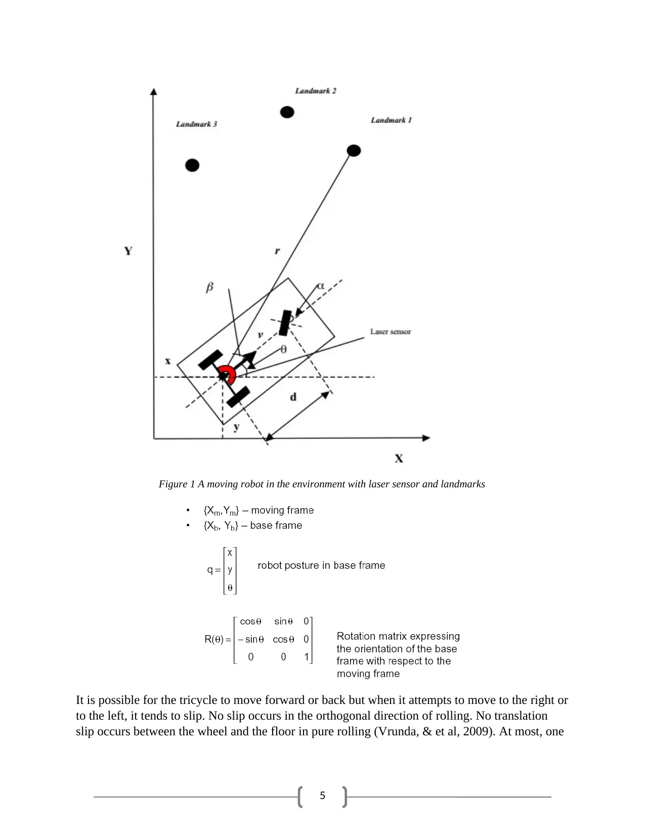
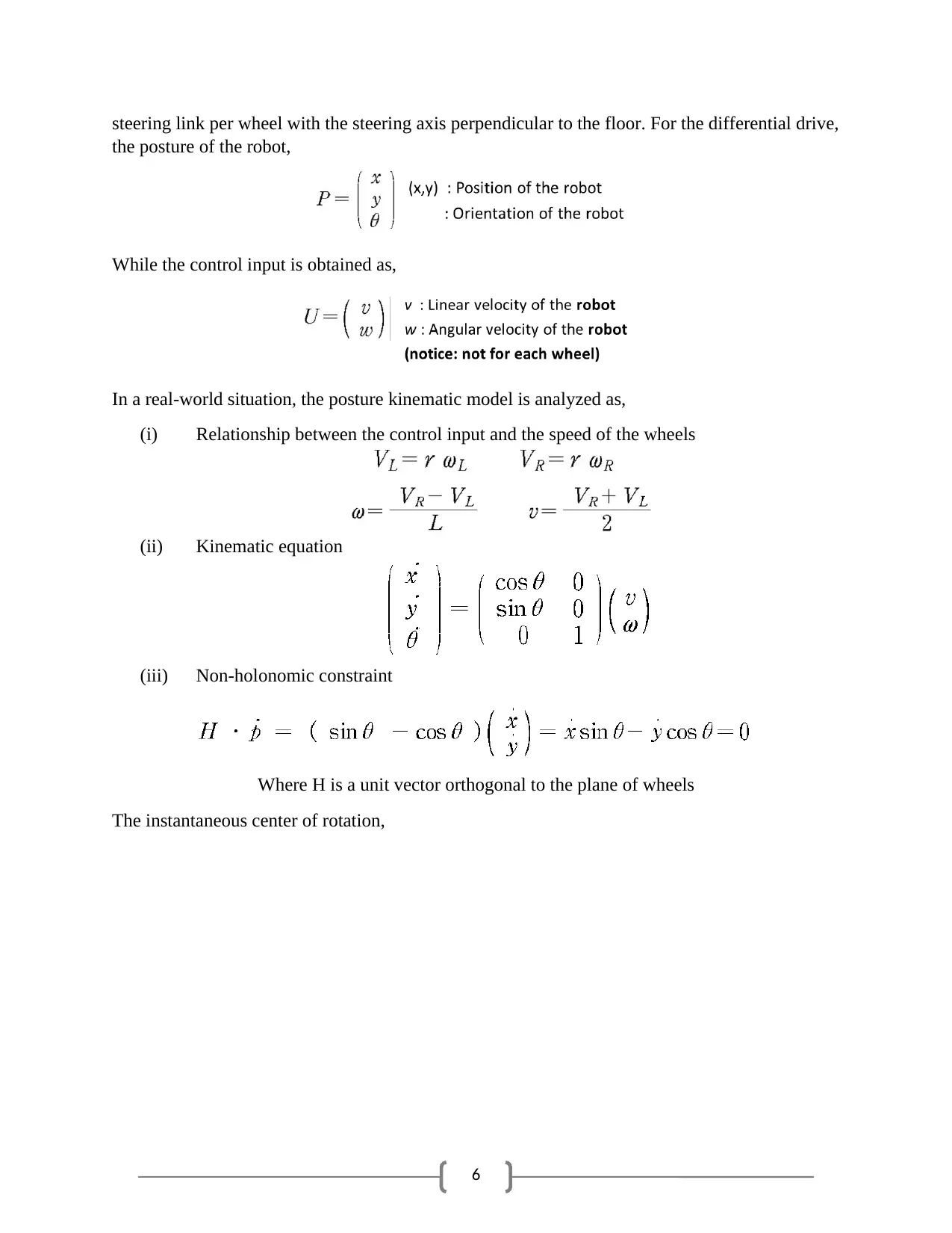
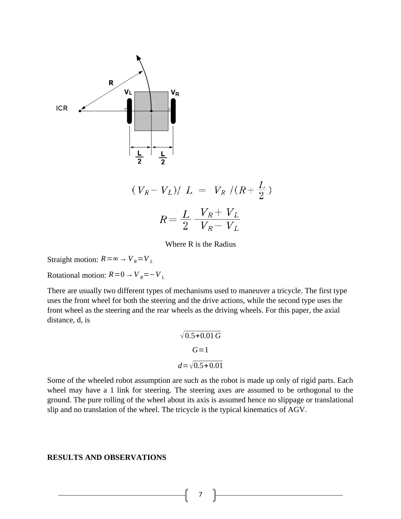
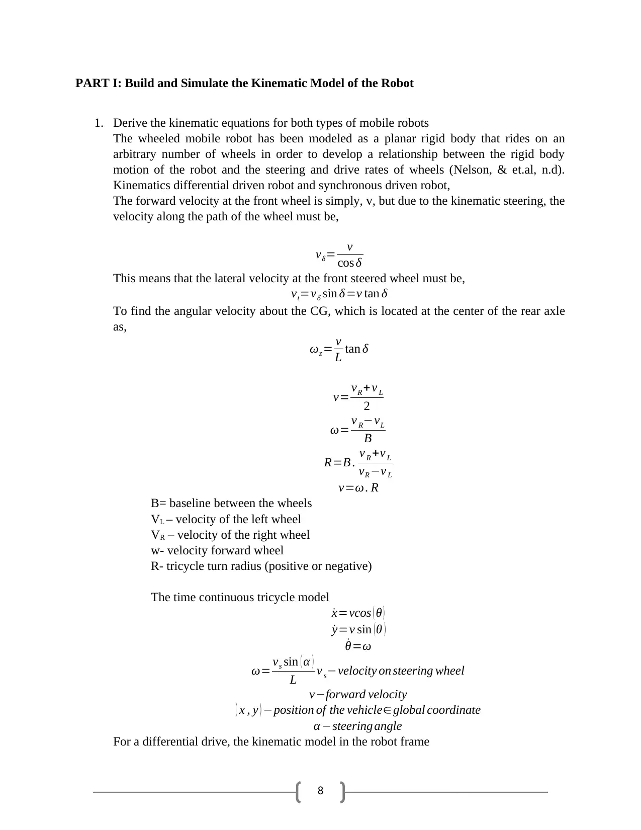
This project delves into the kinematic modeling of a tricycle mobile robot, a three-wheeled vehicle, focusing on its movement capabilities and limitations. The analysis includes deriving kinematic equations for both differential drive and synchronous drive robots, followed by simulations using MATLAB to demonstrate various driving modes, such as constant and linearly changing velocities and steering angles. The project further explores the localization of the tricycle-like robot using a particle filter, providing insights into the robot's position and velocity estimation. The study also compares the results obtained from the two models, discusses the minimum radius of curvature, and highlights the impact of different parameters on the tricycle's path during operation, including the effects of steering angle changes on velocity. Assumptions regarding wheel behavior and sensor measurements are discussed, providing a comprehensive understanding of the tricycle's kinematics and its application in mobile robotics.

1
UNIVERSITY AFFILIATION
DEPARTMENT OR FACULTY
COURSE NAME & CODE
Student ID Student Name % Contribution
PROFESSOR (TUTOR)
DATE OF SUBMISSION

2
ABSTRACT
This paper seeks to review the concept of wheeled mobile robotics using the tricycle. The
tricycle is a three-wheeled vehicle that is able to move forward and back but it encounters a
lateral slip when it moves sideways. The tricycle, in a practical circumstance, encounters the
ground dynamics and hindrances such as friction. In this paper we shall analyze the kinematic
model of the wheeled mobile robot using the tricycle as a case study. A simulation of the
kinematic model of the robots is obtained from the MATLAB toolbox. The simulation
demonstrates different driving modes such as constant driving velocity and a constant steering
angle, constant driving velocity and a linearly changing steering angle, and the linearly changing
driving velocity with linearly changing steering angle (Giovanni, 2009). The three scenarios are
analyzed and discussed. Another simulation is done to view the localization of the tricycle-like
mobile robot using a particle filter. The paper goes further to describe a path that the tricycle
takes during operation to show how the different parameters are affected.

3
TABLE OF CONTENTS
ABSTRACT...............................................................................................................................................2
INTRODUCTION.....................................................................................................................................4
RESULTS AND OBSERVATIONS.........................................................................................................8
DISCUSSION..........................................................................................................................................20
CONCLUSION........................................................................................................................................21
REFERENCES........................................................................................................................................22

4
INTRODUCTION
The tricycle falls under the wheeled robotics in mobile robot locomotion. It is a combination of a
variety of hardware and software components. It manages locomotion, sensing, control,
reasoning, and communication. The tricycle is able to navigate through its environment while it
measures properties of itself and the surrounding. It manages to generate the physical actions and
how the robot maps measurements into actions. A tricycle has three wheels; two rear wheels and
one front wheel. The steering and power are provided through the front wheel and the control
variables are the steering direction and the angular velocity of steering wheel (Dong-Sung, & et
al., 2003). The ICC must lie on the line that passes through and it is orthogonal to the fixed rear
wheels. When the steering wheel is set to an angle from the straight-line direction, the tricycle
will rotate with angular velocity about a point lying a distance R along the line perpendicular to
the passing through of the rear wheels. In a synchronous drive robot, each wheel is capable of
being driven and steered. The three steered wheels are arranged as vertices of an equilateral. The
wheel turn and drive in unison and this leads to a holonomic behavior. All the wheels turn in
unison. The vehicle controls the direction in which the wheels point and the rate at which they
roll. At such a point, all the wheels remain parallel and the synchronous drive always rotates
about the center of the robot (Johann, n.d.). The synchro drive robot has the ability to control the
orientation of their pose directly. In the kinematic modelling, the tricycle falls under
configuration space dim C=4. The kinematic model of the wheeled mobile robot provides all the
feasible directions for the instantaneous motion. It describes the relation between the velocity
input commands and the derivatives of generalized coordinates (a differential model). The
mechanically more complex, steered and driven conventional wheel is utilized on Neptune,
Hero, and Avatar. These three robots have a tricycle wheel arrangement; the front wheel and it is
driven with two rear wheels are at a fixed parallel orientation and are undriven (Nilanjan, & et
al., 2004).
The robots in mobile locomotion communicate with each other or with an outside operator. In
this assignment, one of the key attributes of the tricycle is the kinematics. It is a study of the
mathematics of motion albeit the consideration of the forces that affect the motion. The
kinematics model deals with the geometric relationships that govern the system. It deals with the
relationship between control parameters and the behavior of a system (Kanayama, & et al, n.d).

5
Figure 1 A moving robot in the environment with laser sensor and landmarks
It is possible for the tricycle to move forward or back but when it attempts to move to the right or
to the left, it tends to slip. No slip occurs in the orthogonal direction of rolling. No translation
slip occurs between the wheel and the floor in pure rolling (Vrunda, & et al, 2009). At most, one

6
steering link per wheel with the steering axis perpendicular to the floor. For the differential drive,
the posture of the robot,
While the control input is obtained as,
In a real-world situation, the posture kinematic model is analyzed as,
(i) Relationship between the control input and the speed of the wheels
(ii) Kinematic equation
(iii) Non-holonomic constraint
Where H is a unit vector orthogonal to the plane of wheels
The instantaneous center of rotation,

7
Where R is the Radius
Straight motion: R=∞ → V R =V L
Rotational motion: R=0 →V R=−V L
There are usually two different types of mechanisms used to maneuver a tricycle. The first type
uses the front wheel for both the steering and the drive actions, while the second type uses the
front wheel as the steering and the rear wheels as the driving wheels. For this paper, the axial
distance, d, is
√0.5+0.01 G
G=1
d= √ 0.5+ 0.01
Some of the wheeled robot assumption are such as the robot is made up only of rigid parts. Each
wheel may have a 1 link for steering. The steering axes are assumed to be orthogonal to the
ground. The pure rolling of the wheel about its axis is assumed hence no slippage or translational
slip and no translation of the wheel. The tricycle is the typical kinematics of AGV.
RESULTS AND OBSERVATIONS

8
PART I: Build and Simulate the Kinematic Model of the Robot
1. Derive the kinematic equations for both types of mobile robots
The wheeled mobile robot has been modeled as a planar rigid body that rides on an
arbitrary number of wheels in order to develop a relationship between the rigid body
motion of the robot and the steering and drive rates of wheels (Nelson, & et.al, n.d).
Kinematics differential driven robot and synchronous driven robot,
The forward velocity at the front wheel is simply, v, but due to the kinematic steering, the
velocity along the path of the wheel must be,
vδ= v
cos δ
This means that the lateral velocity at the front steered wheel must be,
vt=vδ sin δ=v tan δ
To find the angular velocity about the CG, which is located at the center of the rear axle
as,
ωz = v
L tan δ
v= vR + v L
2
ω= v R−vL
B
R=B . v R +v L
vR −v L
v=ω . R
B= baseline between the wheels
VL – velocity of the left wheel
VR – velocity of the right wheel
w- velocity forward wheel
R- tricycle turn radius (positive or negative)
The time continuous tricycle model
˙x=vcos ( θ )
˙y=v sin (θ )
˙θ=ω
ω= vs sin ( α )
L v s−velocity on steering wheel
v−forward velocity
( x , y ) −position of the vehicle∈global coordinate
α −steering angle
For a differential drive, the kinematic model in the robot frame

9
[ vx ( t )
v y ( t )
˙θ ( t ) ]=
[ r
2
r
2
0 0
¿ r
L
r
L ]∗
[ω1 ( t )
ωr ( t ) ]
v ( t ) =ω ( t ) R=0.5∗( vr ( t ) + vI ( t ) )
ω ( t )= ( vr ( t ) −v I ( t ) )
L
˙x (t )=v ( t ) cosθ ( t )
˙y ( t ) =v ( t ) sinθ ( t )
˙θ ( t )=ω ( t )
Performing an integral on the values,
We obtain the kinematic equation as,
[ ˙x (t )
˙y (t)
θ(t) ] =
[ cos θ (t) 0
sin θ(t) 0
0 1 ] [ v (t)
w (t) ]
˙q ( t ) =S (q) ξ(t)
2. Simulink to build the kinematic models of the robots and simulate and demonstrate the
behavior of the vehicle subject to
(i) Constant driving velocity and a constant steering angle

10
0 1 2 3 4 5 6 7 8 9 10
Time [s]
0
0.5
1
1.5
Velocity [m/s] RWD vehicle
FWD vehicle
0 1 2 3 4 5 6 7 8 9 10
Time [s]
-0.5
0
0.5
Alpha [rad] RWD vehicle
FWD vehicle
0 1 2 3 4 5 6 7 8 9 10
Time [s]
0
2
4
Theta [rad]
RWD vehicle
FWD vehicle
0 1 2 3 4 5 6 7 8 9 10
Time [s]
0
2
4
Position Y [m]
RWD vehicle
FWD vehicle
0 1 2 3 4 5 6 7 8 9 10
Time [s]
0
1
2
Position X [m]
RWD vehicle
FWD vehicle

11
0 0.5 1 1.5 2
X [m]
0
0.5
1
1.5
2
2.5
3
Y [m]
RWD vehicle
FWD vehicle
(ii) Constant driving velocity and a linearly changing steering angle
0 1 2 3 4 5 6 7 8 9 10
Time [s]
0
0.5
1
1.5
Velocity [m/s] RWD vehicle
FWD vehicle
0 1 2 3 4 5 6 7 8 9 10
Time [s]
-0.5
0
0.5
Steering angle [rad]
RWD vehicle
FWD vehicle

12
0 1 2 3 4 5 6 7 8 9 10
Time [s]
0
1
2
Orientation [rad]
RWD vehicle
FWD vehicle
0 1 2 3 4 5 6 7 8 9 10
Time [s]
0
2
4
Position Y [m]
RWD vehicle
FWD vehicle
0 1 2 3 4 5 6 7 8 9 10
Time [s]
0
2
4
Position X [m]
RWD vehicle
FWD vehicle
0 0.5 1 1.5 2 2.5 3
X [m]
0
0.5
1
1.5
2
2.5
3
Y [m]
RWD vehicle
FWD vehicle