MSc Tunnelling and Underground Space: FEM Design Study Report

This design study report presents a finite element modeling (FEM) analysis for a 4 km tunnel extension to the London metro, focusing on geotechnical considerations in London Clay. The study utilizes Plaxis 2D software to model three cross-sections (A, B, and C) considering varying depths, historical sites with piles, and tunnel dimensions. The report details the selection of cross-sections, model dimensions, tunnel properties (diameter, spacing, lining), and soil profile (London Clay). The Modified Cam-clay model is employed, and structural elements like piles are modeled. The analysis investigates the effects of different tunnel diameters and spacing. The report aims to demonstrate a thorough understanding of FEM methodologies, numerical modeling, and the presentation of results in a clear and replicable manner, providing insights into settlement and impacts on surrounding structures.

1
DESIGN STUDY REPORT

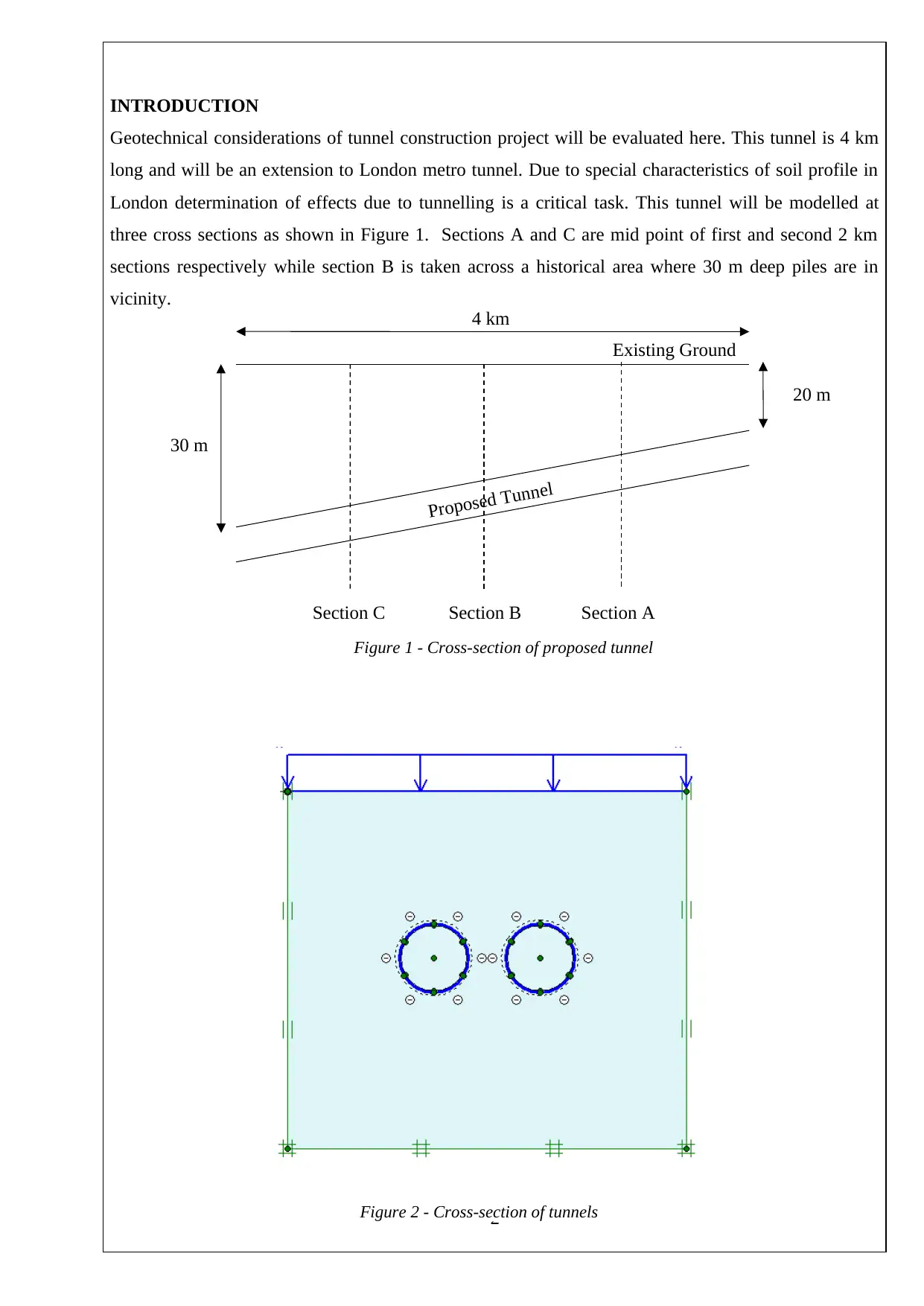
INTRODUCTION
Geotechnical considerations of tunnel construction project will be evaluated here. This tunnel is 4 km
long and will be an extension to London metro tunnel. Due to special characteristics of soil profile in
London determination of effects due to tunnelling is a critical task. This tunnel will be modelled at
three cross sections as shown in Figure 1. Sections A and C are mid point of first and second 2 km
sections respectively while section B is taken across a historical area where 30 m deep piles are in
vicinity.
2
20 m
4 km
30 m
Section C Section B Section A
Proposed Tunnel
Existing Ground
Figure 1 - Cross-section of proposed tunnel
Figure 2 - Cross-section of tunnels

TUNNEL CONSTRUCTION IN LONDON CLAY
Civil Engineers has been conducting researches on London Clay (LC) to identify its properties and to
use it for Engineering applications. London clay has formed by sedimentation of fossils and minerals
during several million years. This special type of clay layer covers most of the part of the capital of
England. This LC is mostly consisted with silt which contributes to the high volumetric change of LC
with the change of Moisture Content (MC) in water.
The city of London is built on this soft clay layer. This clay layer reaches up to 150 m deep from
ground level at some part of London. It is one of main reasons to scarcity of tall buildings in London
city. This LC is not popular for a good bearing capacity. But due to its less permeability it has been an
added advantage to construct tunnels underneath the city of London. This type of soil profile was the
main reason to rapid development of London underground railway Network.
NEW AUSTRIAN TUNNELLING METHOD (NATM)
Tunnel will be constructed in this method by excavating and concreting exposed tunnel. This method
provides a simple approach to tunnel construction with less capital cost, without any complex
construction equipment and processes. Necessity of very skilled work force, Slowness of construction
compared to shield construction, difficulties related to water and require stable soil or rock layers are
some the limitations of this NATM. Since NATM was primarily developed for tunnelling in rocks,
now it is being used with clayey soils. Therefore, it is important to study the behaviour of soils when
tunnelling with NATM (Dasari, Rawlings and Bolton, 1996).
FEM MODELING OF TUNNELS
Various methods have been adopted for tunnelling by different people. Limit state analysis and Limit
equilibrium analysis methods have been used in the past to study the effect on surrounding soil and
structures due to tunnelling. With the evolvement of computer technology use of computers in
Engineering analysis procedures has increased. To analyse these effects using computers Finite
Element Modelling is the most widely used method to idealize the soil and structural elements.
Usually structural elements are idealized by strut, plate and shell element using linear material models
in most of Civil Engineering applications. But when it comes to modelling the soil, it has been used
many constitutive models with different approaches due to complex behaviour of different types of
soils. Mohr – Coulomb model, Soil hardening model, and modified Cam-clay model are few of those
constitutive models.
3

IDEALIZATION OF CONSTRUCTION OF TUNNEL
PLAXIS
Plaxis software will be used to analyse the construction of this tunnel as the Finite Element Modelling
software package. Due to unavailability of Plaxis 3D software Plaxis 2D software was used to analyse
the effect on surroundings due to construction of this 4 km tunnel.
When modelling an actual 3D scenario in to a 2D model various assumptions and techniques must be
used. In Plaxis 2D, Plain Strain and Axe-symmetric idealization methods are available to idealize the
structure. Due to unavailability of Axially symmetric structure Plain strain model was used to idealize
the construction procedure.
SELECTION OF CROSS-SECTIONS
To simulate the actual conditions using plane strain method of idealization a cross section must be
identified. Since this is a considerably long (4 km) construction project 3 cross-sections had to be
modelled to assess settlements and impacts on surrounding structures. Selection of these cross-sections
were done according to the severity of induced effect on the surroundings.
Cross-sections A –
This cross-section was selected at the middle of first 2 km section of the proposed tunnel as shown in
figure 1. It is located at 1 km from the start of the tunnel. Top of the tunnel lining will be located at a
depth of 22.5 m from the existing ground.
Cross-section B –
A historical site and 30 m deep piles were in the vicinity of the proposed tunnel. Since those structures
could be affected by the tunnel construction analysis of this area is a must. Therefore, an analysis
section was selected at the mid point of the section. These historical site and piles are located at a
distance of 2 km from the start of the tunnel. There will be 25 m depth to the top of the lining of the
tunnel from existing ground.
Cross-section C –
This section was selected at the middle of second 2 km section of the proposed tunnel as shown in
figure 1. It is located at 3 km from the start of the tunnel. Top of the tunnel lining will be located at a
depth of 27.5 m from the existing ground.
4

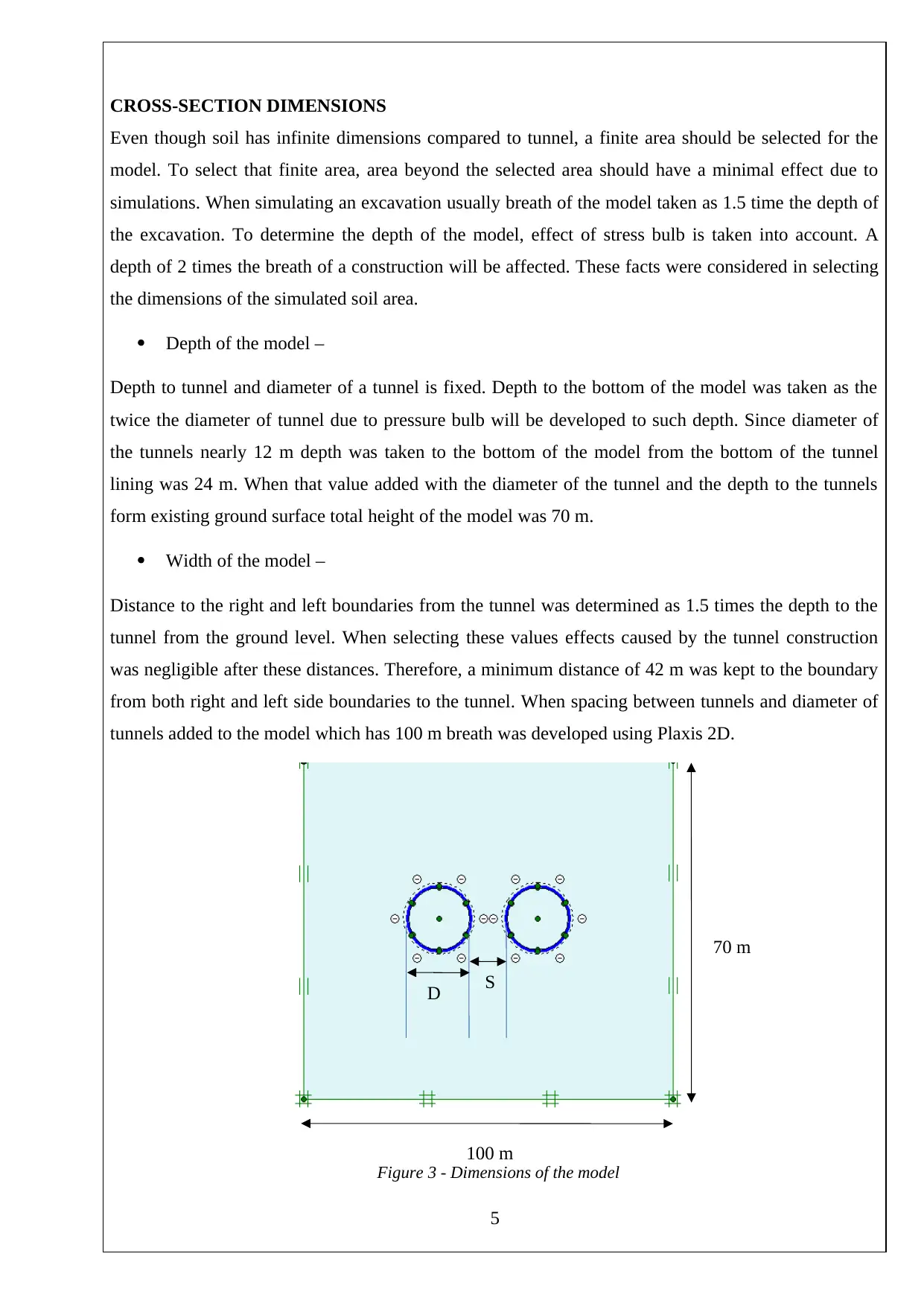
CROSS-SECTION DIMENSIONS
Even though soil has infinite dimensions compared to tunnel, a finite area should be selected for the
model. To select that finite area, area beyond the selected area should have a minimal effect due to
simulations. When simulating an excavation usually breath of the model taken as 1.5 time the depth of
the excavation. To determine the depth of the model, effect of stress bulb is taken into account. A
depth of 2 times the breath of a construction will be affected. These facts were considered in selecting
the dimensions of the simulated soil area.
 Depth of the model –
Depth to tunnel and diameter of a tunnel is fixed. Depth to the bottom of the model was taken as the
twice the diameter of tunnel due to pressure bulb will be developed to such depth. Since diameter of
the tunnels nearly 12 m depth was taken to the bottom of the model from the bottom of the tunnel
lining was 24 m. When that value added with the diameter of the tunnel and the depth to the tunnels
form existing ground surface total height of the model was 70 m.
 Width of the model –
Distance to the right and left boundaries from the tunnel was determined as 1.5 times the depth to the
tunnel from the ground level. When selecting these values effects caused by the tunnel construction
was negligible after these distances. Therefore, a minimum distance of 42 m was kept to the boundary
from both right and left side boundaries to the tunnel. When spacing between tunnels and diameter of
tunnels added to the model which has 100 m breath was developed using Plaxis 2D.
5
70 m
100 m
D S
Figure 3 - Dimensions of the model

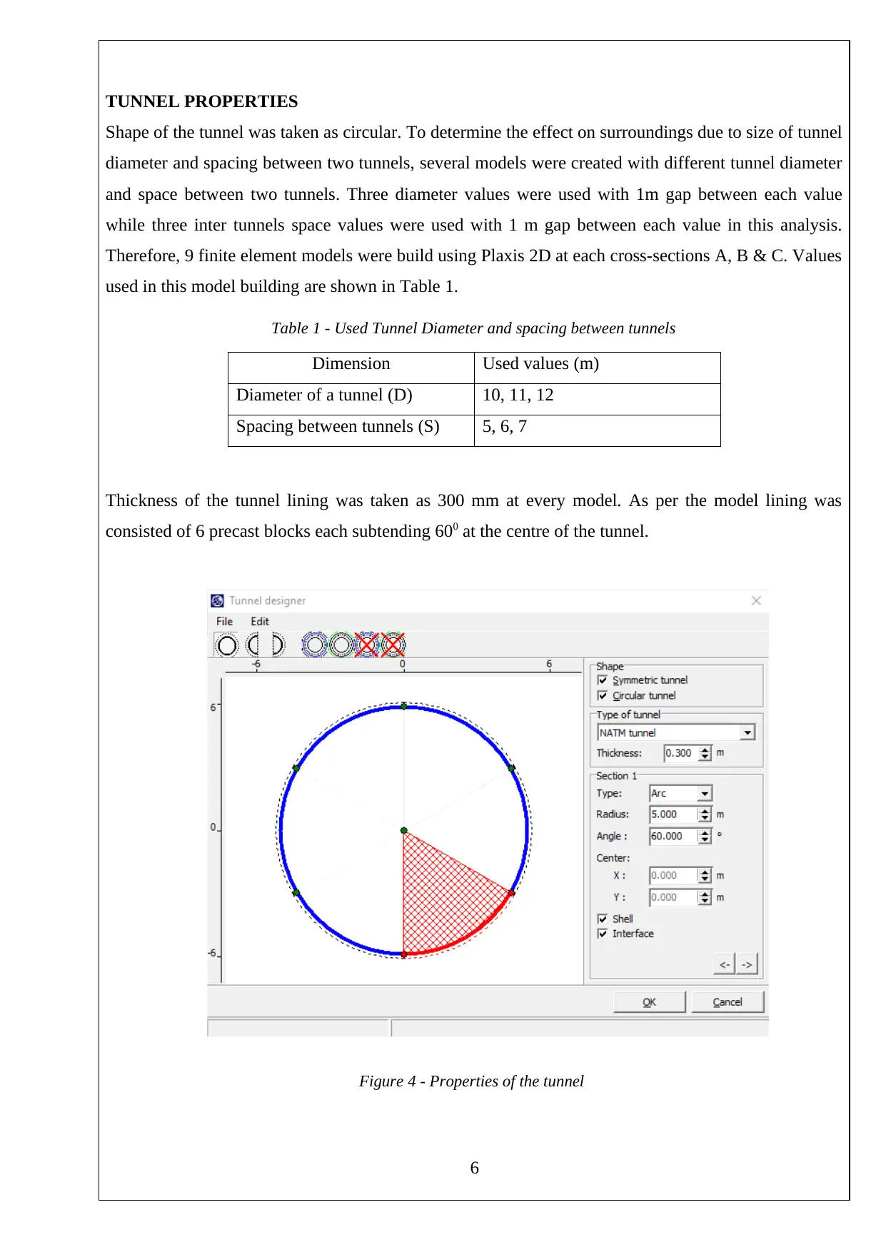
TUNNEL PROPERTIES
Shape of the tunnel was taken as circular. To determine the effect on surroundings due to size of tunnel
diameter and spacing between two tunnels, several models were created with different tunnel diameter
and space between two tunnels. Three diameter values were used with 1m gap between each value
while three inter tunnels space values were used with 1 m gap between each value in this analysis.
Therefore, 9 finite element models were build using Plaxis 2D at each cross-sections A, B & C. Values
used in this model building are shown in Table 1.
Table 1 - Used Tunnel Diameter and spacing between tunnels
Dimension Used values (m)
Diameter of a tunnel (D) 10, 11, 12
Spacing between tunnels (S) 5, 6, 7
Thickness of the tunnel lining was taken as 300 mm at every model. As per the model lining was
consisted of 6 precast blocks each subtending 600 at the centre of the tunnel.
6
Figure 4 - Properties of the tunnel

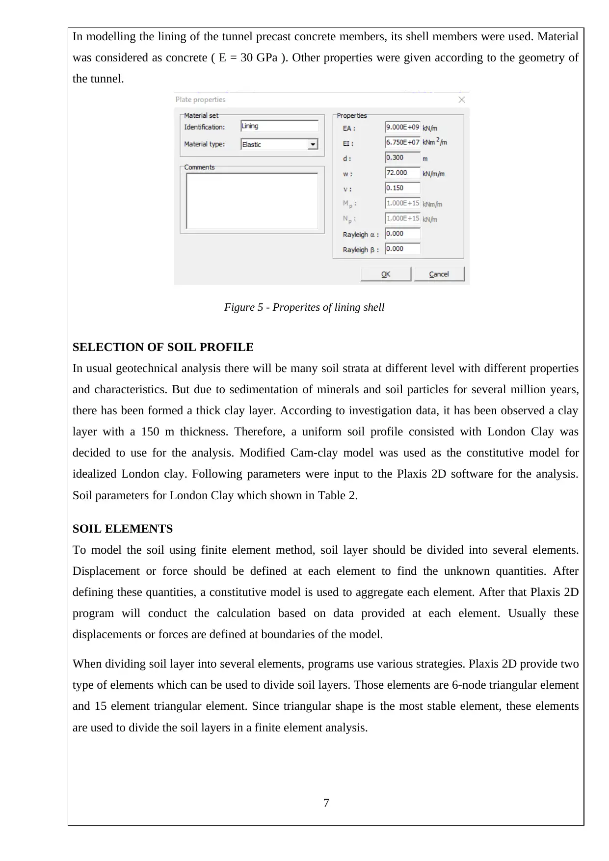
In modelling the lining of the tunnel precast concrete members, its shell members were used. Material
was considered as concrete ( E = 30 GPa ). Other properties were given according to the geometry of
the tunnel.
SELECTION OF SOIL PROFILE
In usual geotechnical analysis there will be many soil strata at different level with different properties
and characteristics. But due to sedimentation of minerals and soil particles for several million years,
there has been formed a thick clay layer. According to investigation data, it has been observed a clay
layer with a 150 m thickness. Therefore, a uniform soil profile consisted with London Clay was
decided to use for the analysis. Modified Cam-clay model was used as the constitutive model for
idealized London clay. Following parameters were input to the Plaxis 2D software for the analysis.
Soil parameters for London Clay which shown in Table 2.
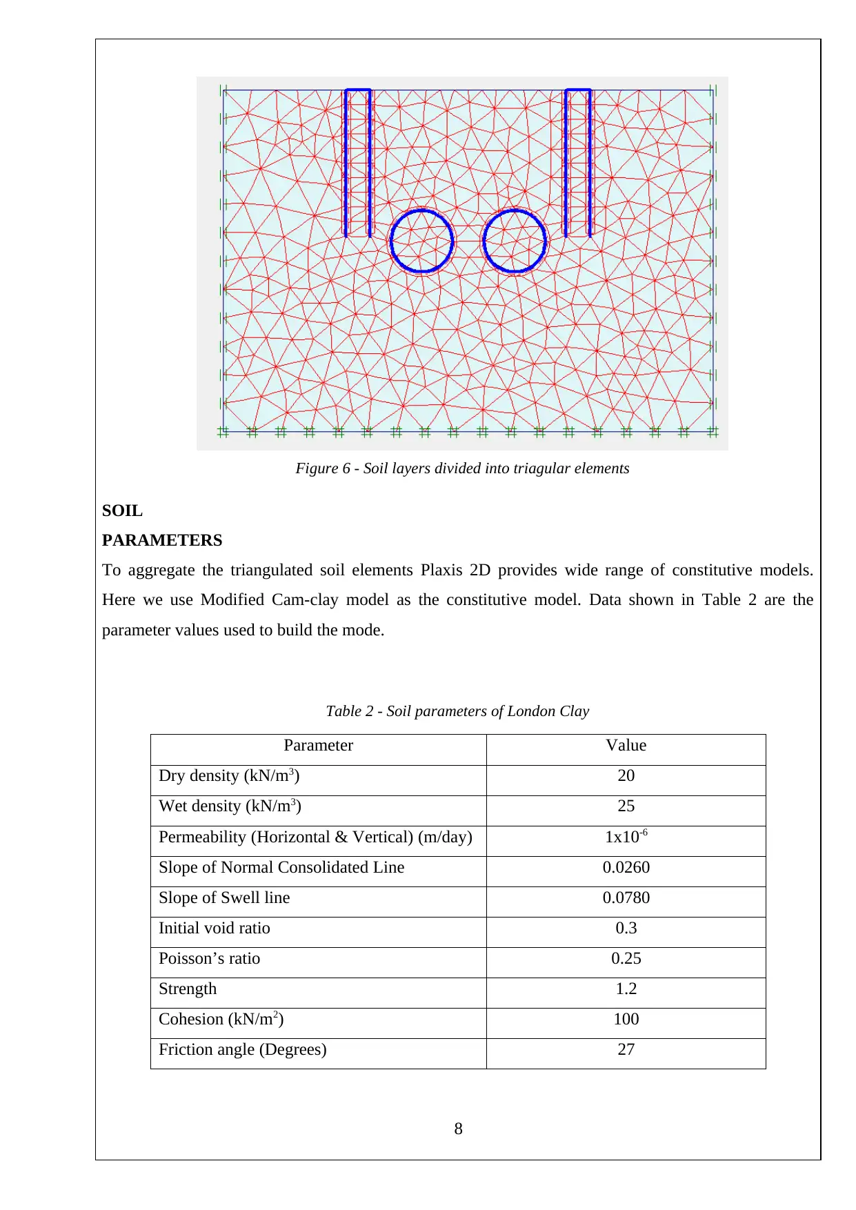
SOIL ELEMENTS
To model the soil using finite element method, soil layer should be divided into several elements.
Displacement or force should be defined at each element to find the unknown quantities. After
defining these quantities, a constitutive model is used to aggregate each element. After that Plaxis 2D
program will conduct the calculation based on data provided at each element. Usually these
displacements or forces are defined at boundaries of the model.
When dividing soil layer into several elements, programs use various strategies. Plaxis 2D provide two
type of elements which can be used to divide soil layers. Those elements are 6-node triangular element
and 15 element triangular element. Since triangular shape is the most stable element, these elements
are used to divide the soil layers in a finite element analysis.
7
Figure 5 - Properites of lining shell

SOIL
PARAMETERS
To aggregate the triangulated soil elements Plaxis 2D provides wide range of constitutive models.
Here we use Modified Cam-clay model as the constitutive model. Data shown in Table 2 are the
parameter values used to build the mode.
Table 2 - Soil parameters of London Clay
Parameter Value
Dry density (kN/m3) 20
Wet density (kN/m3) 25
Permeability (Horizontal & Vertical) (m/day) 1x10-6
Slope of Normal Consolidated Line 0.0260
Slope of Swell line 0.0780
Initial void ratio 0.3
Poisson’s ratio 0.25
Strength 1.2
Cohesion (kN/m2) 100
Friction angle (Degrees) 27
8
Figure 6 - Soil layers divided into triagular elements

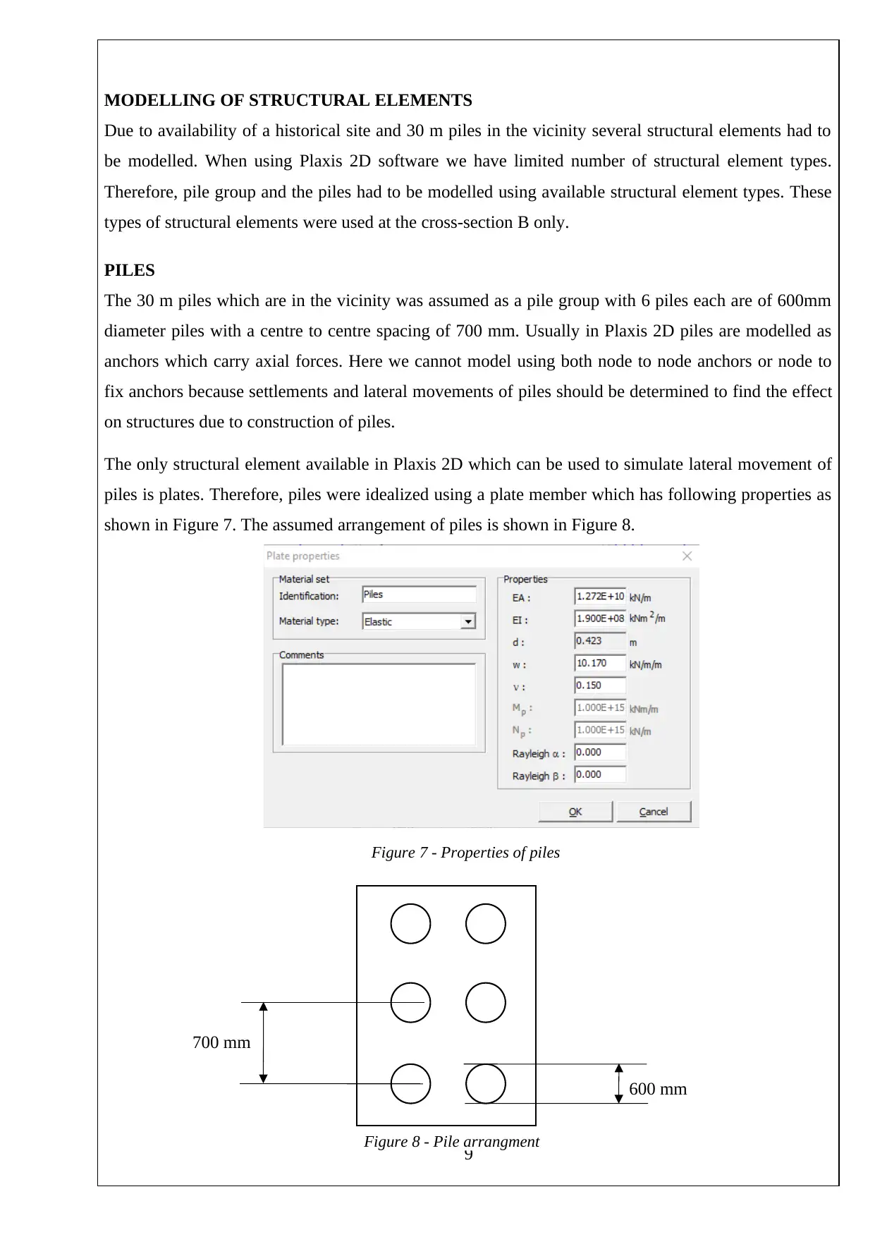
MODELLING OF STRUCTURAL ELEMENTS
Due to availability of a historical site and 30 m piles in the vicinity several structural elements had to
be modelled. When using Plaxis 2D software we have limited number of structural element types.
Therefore, pile group and the piles had to be modelled using available structural element types. These
types of structural elements were used at the cross-section B only.
PILES
The 30 m piles which are in the vicinity was assumed as a pile group with 6 piles each are of 600mm
diameter piles with a centre to centre spacing of 700 mm. Usually in Plaxis 2D piles are modelled as
anchors which carry axial forces. Here we cannot model using both node to node anchors or node to
fix anchors because settlements and lateral movements of piles should be determined to find the effect
on structures due to construction of piles.
The only structural element available in Plaxis 2D which can be used to simulate lateral movement of
piles is plates. Therefore, piles were idealized using a plate member which has following properties as
shown in Figure 7. The assumed arrangement of piles is shown in Figure 8.
9
Figure 7 - Properties of piles
600 mm
700 mm
Figure 8 - Pile arrangment

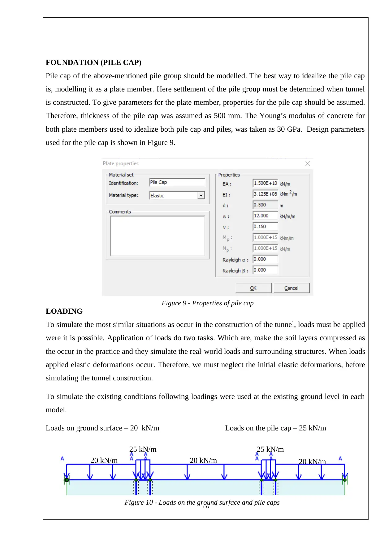
FOUNDATION (PILE CAP)
Pile cap of the above-mentioned pile group should be modelled. The best way to idealize the pile cap
is, modelling it as a plate member. Here settlement of the pile group must be determined when tunnel
is constructed. To give parameters for the plate member, properties for the pile cap should be assumed.
Therefore, thickness of the pile cap was assumed as 500 mm. The Young’s modulus of concrete for
both plate members used to idealize both pile cap and piles, was taken as 30 GPa. Design parameters
used for the pile cap is shown in Figure 9.
LOADING
To simulate the most similar situations as occur in the construction of the tunnel, loads must be applied
were it is possible. Application of loads do two tasks. Which are, make the soil layers compressed as
the occur in the practice and they simulate the real-world loads and surrounding structures. When loads
applied elastic deformations occur. Therefore, we must neglect the initial elastic deformations, before
simulating the tunnel construction.
To simulate the existing conditions following loadings were used at the existing ground level in each
model.
Loads on ground surface – 20 kN/m Loads on the pile cap – 25 kN/m
10
Figure 9 - Properties of pile cap
20 kN/m
25 kN/m
20 kN/m20 kN/m
25 kN/m
Figure 10 - Loads on the ground surface and pile caps

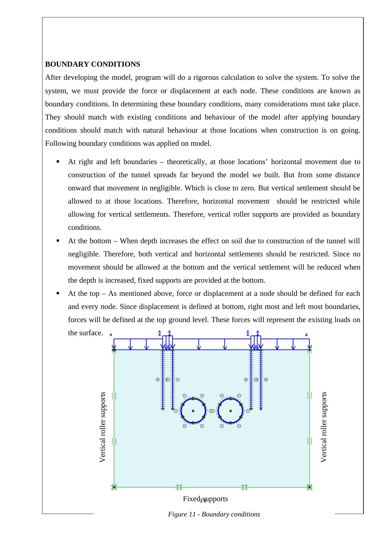
BOUNDARY CONDITIONS
After developing the model, program will do a rigorous calculation to solve the system. To solve the
system, we must provide the force or displacement at each node. These conditions are known as
boundary conditions. In determining these boundary conditions, many considerations must take place.
They should match with existing conditions and behaviour of the model after applying boundary
conditions should match with natural behaviour at those locations when construction is on going.
Following boundary conditions was applied on model.
 At right and left boundaries – theoretically, at those locations’ horizontal movement due to
construction of the tunnel spreads far beyond the model we built. But from some distance
onward that movement in negligible. Which is close to zero. But vertical settlement should be
allowed to at those locations. Therefore, horizontal movement should be restricted while
allowing for vertical settlements. Therefore, vertical roller supports are provided as boundary
conditions.
 At the bottom – When depth increases the effect on soil due to construction of the tunnel will
negligible. Therefore, both vertical and horizontal settlements should be restricted. Since no
movement should be allowed at the bottom and the vertical settlement will be reduced when
the depth is increased, fixed supports are provided at the bottom.
 At the top – As mentioned above, force or displacement at a node should be defined for each
and every node. Since displacement is defined at bottom, right most and left most boundaries,
forces will be defined at the top ground level. These forces will represent the existing loads on
the surface.
11
Vertical roller supports
Fixed supports
Vertical roller supports
Figure 11 - Boundary conditions

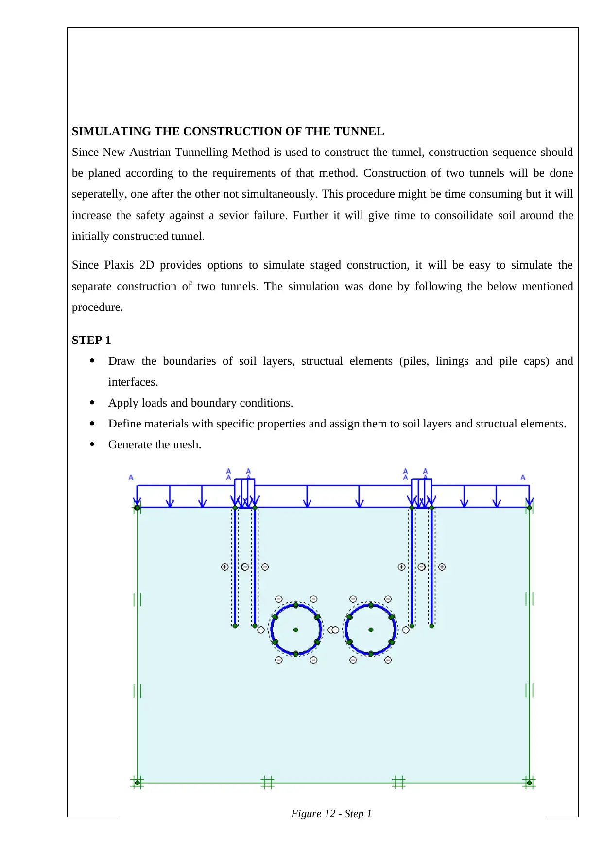
SIMULATING THE CONSTRUCTION OF THE TUNNEL
Since New Austrian Tunnelling Method is used to construct the tunnel, construction sequence should
be planed according to the requirements of that method. Construction of two tunnels will be done
seperatelly, one after the other not simultaneously. This procedure might be time consuming but it will
increase the safety against a sevior failure. Further it will give time to consoilidate soil around the
initially constructed tunnel.
Since Plaxis 2D provides options to simulate staged construction, it will be easy to simulate the
separate construction of two tunnels. The simulation was done by following the below mentioned
procedure.
STEP 1
 Draw the boundaries of soil layers, structual elements (piles, linings and pile caps) and
interfaces.
 Apply loads and boundary conditions.
 Define materials with specific properties and assign them to soil layers and structual elements.
 Generate the mesh.
12
Figure 12 - Step 1

STEP 2
 Insert water table level at 5 m.
 Calculate pore water preassures and earth pressure coefficients.
STEP 3
 Elastic settlements due to applied loads should be negelected. Therefore, loads on ground level
and pile caps are applied first and there settlement is neglected in tunnel construction steps.
 Activate
loads,
pile and pile
caps in this
step.
13
Figure 13 - Step 2

STEP 4
 Define new step and reset displacements to zero.
 Activate one tunnel lining and deactivate the soil inside it.
STEP 5
 Activate
the lining of
the remaining
lining.
14
Figure 15 - Step 4 (Activate one tunnel lining)

FINAL CORSS SETION DATA
SECTION A
This section is located in first 2 km of the tunnel. Therefore, top of the tunnel is located at 22.5 m from
the ground level. No piles or piles caps are in vicinity.
SECTION B
Since piles and the
historic site are in
vicinity.
15
Figure 17 - Section A

Therefore, loads and features change in the section. Tunnels are located in 25 m below the ground
level.
SECTION C
This section is very simillar to section A but depth to the tunnel top will be 27.5 m from the ground
level.
RESULTS
27 finite element models were created for each diameter and space between tunnel combination. In the
analysis of resutls most critical section is section B. Because it consit with several important structual
16
Figure 18 - Section B
Figure 19 - Section C

elements. But other two section are also important when evaluating the effects on surroundings due to
the construction of the tunnel.
Therefore, effect on surroundings at each section when diameter and spacing changes are determined
here. In determining the effect, following parameters will be considered.
 Ground level settlement
 Settelment under the lining of the tunnel
 Axial forces in tunnel lining
 Maximum deformation in tunnel lining
 Settlement of pile cap
 Vertical settlement and lateral deformation of piles.
Settelment of piles and pile caps will be conducted only for the cross section B. Other cross sections
does not include those elements.
GROUND LEVEL SETTLEMENT
Since activities conducted on ground surface will be hevealy dependant on the settlement induced by
the construction of tunnels, those settlements should be analysed properly. According to the finite
element model build using Plaxis 2D the following results were observed at the ground level.
17
Figure 20 - Vertical deformation caused due to tunnel construction

Settlements induced on ground level by construction of two tunnels are represented in following table
seperately. Variation in ground settlement was analysed with restpect to the diameter of the tunnel and
spacing between the tunnels for each section.
Table 3 - Settlement in Existing Ground
Ground level settlement (mm)
Section A B C
Diameter of the tunnel
(m)
Spacing between
Tunnels (m)
Due
tunnel
1
Due
Tunnel
2
Due
Tunnel
2
Due
Tunnel
2
Due
tunnel
1
Due
Tunnel
2
10
5 55.84 95.83 59.4 102.9 44.1 79.3
6 53.12 95.82 61.3 90.5 42.3 74.5
7 54.1 95.83 62.8 89.2 44.1 76.8
11
5 38.4 77.99 60.74 96.1 43.5 77.07
6 52.1 91.2 62.3 88.35 43.6 75.9
7 40.3 77.2 70.5 107.3 43.3 83.2
12
5 51.4 88.2 46.7 80.2 42.2 82.1
6 50.4 85.6 60.3 82.6 42.4 72.5
7 50.3 83.4 47.2 81.3 42.1 70.8
Grapical representation of settlement in ground level as follows with respect to the location in the
model.
SECTION A
Variation in with respect to the diameter of the tunnel is same for both tunnels. Settlement due to 10m
diameter tunnel is large with respect to other two tunnels. Less distance to the ground surface from a
10 m diameter tunnel might be a reason for that issue. When the spacing between two tunnels is 6m,
18
4 5 6 7 8
30
40
50
60
70
80
90
100
10 m due to tunnel 1
11 m due to tunnel 1
12 m due to tunne 1
10 m due to tunnel 2
11 m due to tunnel 2
12 m due to tunnel 2
Tunnel spacing (m)
Settlement (mm)
Figure 21 - Ground level settlement at Section A

ground settlement becomes less with respect to other spacing valuse in 10 m and 12 m diameter
tunnels but ground settlement will be high with a 11 m diameter tunnels are constructed with 6m
spacing.
SECTION B
4 5 6 7 8
30
40
50
60
70
80
90
100
110
120
10 m due to tunnel 1
11 m due to tunnel 1
12 m due to tunne 1
10 m due to tunnel 2
11 m due to tunnel 2
12 m due to tunnel 2
Tunnel spacing (m)
Settlement (mm)
Figure 22 - Ground level settlement at Section B
SECTION C
4 5 6 7 8
30
40
50
60
70
80
90
10 m due to tunnel 1
11 m due to tunnel 1
12 m due to tunne 1
10 m due to tunnel 2
11 m due to tunnel 2
12 m due to tunnel 2
Tunnel spacing (m)
Settlement (mm)
Settlement variation in both Section B and Section C are similar as the section A. But in section C
variation with respect to the tunnel diamete is very less. Deepness of the tunnel location might be this
little varation in ground level. Values observed at Section B is compartive high than both A & B
sections. Applied loads on section B is high than other two sections.
19

SETTLEMENT UNDER LINING
Table 4 - Settlement under lining
Settlement under lining (mm)
Section A B C
Diameter of the tunnel
(m)
Spacing between
Tunnels (m)
Due
tunnel
1
Due
Tunnel
2
Due
Tunnel
2
Due
Tunnel
2
Due
tunnel
1
Due
Tunnel
2
10
5 65.2 67.1 50.1 55.6 51.7 62.4
6 53 57.1 46.1 61.5 45.3 59.8
7 55.81 57.3 51.1 57 46.2 60.3
11
5 50.4 63.5 39.4 50.5 43.7 56.1
6 53.8 66.1 43.2 53.1 43.64 52.6
7 52.5 64.1 42.1 53.3 44.6 48.8
12
5 55.3 71.2 38.3 53.3 40.5 44.1
6 50.19 59.1 43.8 53.1 40.5 48.4
7 47.2 59.4 43.9 46.3 41.5 48.6
Settlement under lining should be minimized in tunnel construction. Because excessive settlement
might cause differential settlements in tunnel which might lead to fracturing in lining.
Settlement variation is represented in graphical form as follows.
SECTION A
Figure 23 - Settlement under the lining at Section A
SECTION B
20
4 5 6 7 8
45
50
55
60
65
70
75
10 m due to tunnel 1
11 m due to tunnel 1
12 m due to tunne 1
10 m due to tunnel 2
11 m due to tunnel 2
12 m due to tunnel 2
Tunnel spacing (m)
Settlement (mm)
35
40
45
50
55
60
65
10 m due to tunnel 1
11 m due to tunnel 1
12 m due to tunne 1
10 m due to tunnel 2
11 m due to tunnel 2
12 m due to tunnel 2
Settlement (mm)

SECTION C
4 5 6 7 8
35
40
45
50
55
60
65
10 m due to tunnel 1
11 m due to tunnel 1
12 m due to tunne 1
10 m due to tunnel 2
11 m due to tunnel 2
12 m due to tunnel 2
Tunnel spacing (m)
Settlement (mm)
Figure 25 - Settlement under the lining at Section C
AXIAL FORCE IN THE LINING
Since lining is constructed using concrete, forces acting on it should not exceed the capacity of the
material. If not, it will cause several issues in tunnel intergrity. Axial forces determined using finite
element model with respect to the section, tunnel diameter and the spacing between the tunnels are
shown in Table 5.
Table 5 - Axial forces in lining with respect to location
Axial force in lining (kN/m)
Section A B C
Diameter of the tunnel
(m)
Spacing between
Tunnels (m)
Due
tunnel
1
Due
Tunnel
2
Due
Tunnel
2
Due
Tunnel
2
Due
tunnel
1
Due
Tunnel
2
10
5 2040 2070 2190 2200 2320 2350
6 2040 2060 2200 2230 2320 2340
7 2040 2060 2200 2230 2320 2340
11 5 2310 2280 2440 2450 2570 2600
6 2260 2290 2440 2470 2570 2600
21
Tunnel spacing (m)
Figure 24 - Settlement under the lining at Section B

7 2290 2280 2380 2450 2570 2570
12
5 2090 2120 2690 2470 2830 2830
6 2490 2520 2690 2730 2830 2860
7 2490 2520 2680 2730 2830 2860
As shown in following Figure 26, Figure 27 and Figure 27 the variation of axial force does not
critically varies with the diameter of the tunnel. But it will drastically change with the depth to the
tunnel lining. Variation in axial force is graphically represented by following figures.
SECTION A
4 5 6 7 8
2000
2100
2200
2300
2400
2500
2600
10 m due to tunnel 1
11 m due to tunnel 1
12 m due to tunne 1
10 m due to tunnel 2
11 m due to tunnel 2
12 m due to tunnel 2
Tunnel spacing (m)
Axial Force (kN/m)
Figure 26 - Axial force in tunnel lining at Section A
SECTION B
4 5 6 7 8
2000
2100
2200
2300
2400
2500
2600
2700
2800
10 m due to tunnel 1
11 m due to tunnel 1
12 m due to tunne 1
10 m due to tunnel 2
11 m due to tunnel 2
12 m due to tunnel 2
Tunnel spacing (m)
Axial force (kN/m)
Figure 27 - Axial force on tunnel lining at Section B
22

SECTION C
4 5 6 7 8
2100
2200
2300
2400
2500
2600
2700
2800
2900
10 m due to tunnel 1
11 m due to tunnel 1
12 m due to tunne 1
10 m due to tunnel 2
11 m due to tunnel 2
12 m due to tunnel 2
Tunnel spacing (m)
Axial force (kN/m)
Figure 28 - Axial force on tunnel lining at Section C
DEFORMATION OF THE TUNNEL LINING
Deformations in the tunnel lining is another important partmeter which should be constidered in
designing the tunnel. If deformations are greater than the specified values, tunnel may not be in service
conditions. Lining deformations can be determined using Plaxis 2D. Here, only vertical deformations
are evaluated.
Table 6 shows the vertical deformation of linings with respect to the tunnel diameter, spacing of two
tunnels and the section.
Table 6 - Vertical Deformation of tunnel linings
Deformation (mm)
Section A B C
Diameter of the tunnel
(m)
Spacing between
Tunnels (m)
Due
tunnel
1
Due
Tunnel
2
Due
Tunnel
2
Due
Tunnel
2
Due
tunnel
1
Due
Tunnel
2
10
5 171.2 181.5 158.1 148.2 152.1 163.5
6 170 184.5 159 171.2 180.1 162.3
7 170.2 191.2 160.1 169.9 152.1 161.5
11
5 167.2 165.9 145.1 151.2 138.4 148.1
6 151.2 166.2 146.1 155.2 138.4 144.1
7 149.3 164.3 122.1 134.9 138.1 124.6
12
5 166.4 177.1 126.2 137.1 124.3 122.6
6 139.5 148.1 133.2 136.1 123.5 131.8
7 138.4 147.5 126.3 136.4 124.5 130.8
23

Following graphs illustarate the variation of the deformation of the tunnel diameter of each section.
SECTION A
SECTION B
4 5 6 7 8
120
130
140
150
160
170
180
10 m due to tunnel 1
11 m due to tunnel 1
12 m due to tunne 1
10 m due to tunnel 2
11 m due to tunnel 2
12 m due to tunnel 2
Tunnel spacing (m)
Vertical Deformation (mm)
Figure 30 - Vertical deformation in lining at Section B
24
4 5 6 7 8
130
140
150
160
170
180
190
200
10 m due to tunnel 1
11 m due to tunnel 1
12 m due to tunne 1
10 m due to tunnel 2
11 m due to tunnel 2
12 m due to tunnel 2
Tunnel spacing (m)
Vertical deformation (mm)
Figure 29 - Vertical deformation in lining at Section A

SECTION C
4 5 6 7 8
120
130
140
150
160
170
180
10 m due to tunnel 1
11 m due to tunnel 1
12 m due to tunne 1
10 m due to tunnel 2
11 m due to tunnel 2
12 m due to tunnel 2
Tunnel spacing (m)
Veertical deformation (mm)
Figure 31 - Vertical deformation in lining at Section C
SETTLEMENT IN PILE CAP
At historic site the effects due to the construction of tunnels should be minimized. Therefroe
settelments in the structures should be minimised. Plaxis 2d povides facilities to predict the settlements
which may occur during the construction. Settement data obtained form the model as follows.
Table 7 - Settlements in Pile cap
Deformation (mm)
Diameter of the tunnel
(m)
Spacing
between
Tunnels (m)
Due
tunnel 1
Due
Tunnel
2
10
5 24.8 35.9
6 25.9 34.4
7 26.4 35.1
11
5 25.5 33.8
6 25.8 34.1
7 28.9 37.7
12
5 24.9 32.8
6 24.8 32.1
7 26.5 33.7
25

SETTLEMENT IN PILES
At historic site the effects due to the construction of tunnels should be minimized. Therefroe
settelments in the structures should be minimised. Plaxis 2d povides facilities to predict the settlements
which may occur during the construction. Settement data obtained form the model as follows.
Deformation (mm)
Diameter of the tunnel
(m)
Spacing
between
Tunnels (m)
Due
tunnel 1
Due
Tunnel
2
10
5 24.8 35.9
6 25.9 34.4
7 26.4 35.1
11
5 25.5 33.8
6 25.8 34.1
7 28.9 37.7
12
5 24.9 32.8
6 24.8 32.1
7 26.5 33.7
26
4 5 6 7 8
22
24
26
28
30
32
34
36
38
10 m due to tunnel 1
11 m due to tunnel 1
12 m due to tunne 1
10 m due to tunnel 2
11 m due to tunnel 2
12 m due to tunnel 2
Tunnel spacing (m)
Settlement (mm)

USE OF A DIFFERENT CONSTITUTIVE MODEL
To predict the behaviour of soils, researchers have proposed many constitutive models in combining
the divided soil element when modeling with finite element modeling. Since behaviour of soil is a
complex task. Therefore, each constitutive model has advantages and disadvantages over the others.
Each constitutive model accurately predict the behaviour of soils for a certain range and predictions
diviate from actual failure parameters as the pass that range.
Mohr-Coulomb model and modified Cam-clay model are commonly used constitutive models. Each
model has its own advantages and limitations in modelling the behaviour of soils.
MOHR-COULOMB CONSTITUTIVE MODEL
27
4 5 6 7 8
0
5
10
15
20
25
30
10 m due to tunnel
1
11 m due to tunnel
1
12 m due to tunne 1
10 m due to tunnel
2
Tunnel spacing (m)
Settlement (mm)

This Mohr-Coulomb model is an elastic- perfectly plastic model which is used to model soil behaviour
oftenly. In this model stress – strain behaviour modeled linearly in the elastic range using two
parameters, Young’s modulus (E) and Poisson’s ratio (v). To determine the failure criteria friction
angle and cohesion is used.
This model is simple and applicable for three-dimensional stresses as well. Regarding its strength
behaviour, this model performs better. This model can be used to analyse the stability of dams, slopes,
embankments and shallow foundations. Although failure behaviour is generally well captured in
drained conditions, the effective stress path that is followed in undrained materials may deviate
significantly, from observations.
MODIFIED CAM-CLAY MODEL
The Modified Cam-clay is an elastic plastic strain hardening model where the non-linear behaviour is
modelled by means of hardening plasticity. The model is based on Critical State theory and the basic
assumption that there is a logarithmic relationship between the mean effective stress, p’ and the void
ratio, e. Virgin compression and recompression lines are linear in the e-ln p’ space, which is most
realistic for near-normally consolidated clays. Only linear elastic behaviour is modelled before
yielding and may results in unreasonable values of ν due to log-linear compression lines.
This model is more suitable to describe deformation than failure especially for normally consolidated
soft soils. The model also performs best in applications involving loading conditions such as
embankment or foundation. It involves four parameters, i.e. the isotropic logarithmic compression
index, λ, the swelling index, κ, Poisson’s ratio for unloading and reloading, νur, friction constant, M,
pre-consolidation stress, pc and the initial void ratio, e. Shear strength can only be modeled using the
effective friction constant. In the case of primary undrained deviatoric loading of soft soils, the model
predicts more realistic undrained shear strength compared to the Mohr-Coulomb model. In addition to
achieve better agreement between predicted and observed soil behaviour, a large number of
modifications have been proposed to the standard Cam-clay models over the last two decades.
identified the limitations of this model. The yield surfaces adopted in many critical state models
significantly overestimate failure stresses on the ‘dry side’. These models assumed an associated flow
rule and therefore were unable to predict an important feature of behaviour that is commonly observed
in undrained tests on loose
sand and normally
consolidated undisturbed
clays, and that is a peak in
28
Figure 34 - Stress-Strain relationship of Mohr-Coulomb model

the deviatoric stress before the critical state is approached. The critical state had been much less
successful for modeling granular materials due to its inability to predict observed softening and
dilatancy of dense sands and the undrained response of very loose sands. where it is also noted that the
materials modeled by critical state models appeared to be mostly limited to saturated clays and silts,
and stiff overconsolidated clays did not appear to be generally modeled with critical state formulations.
Modified Cam-Clay model can be used to analyse soft clay, silty soils and normally consolidated clay.
In this simulation usage of Mohr-Coulumb may not be suitable because beahaviour of London Clay
does not cannot be simulated accurately by using that model. Non linear behaviour of London clay can
be modelled approximated by the Cam-Clay model.
Values predicted by Cam caly model might differ with values predicted by a model which used Mohr-
Coulomb model.
29
Figure 35 - Relationship between e and log(p)