BTM7104 Statistics I: Analyzing Factors Affecting Two-Wheeler Sales
VerifiedAdded on 2023/06/04
|20
|4126
|326
Report
AI Summary
This report presents a fictitious study using imaginary data to explore the relationship between the two-wheeler automobile industry and macroeconomic factors. It investigates the impact of GDP growth rate and unemployment rates on the sales volume of two-wheeled vehicles. The study formulates two hypotheses: a positive correlation between GDP growth and sales volume, and a negative correlation between unemployment rates and sales volume. The data, consisting of 33 observations, undergoes descriptive analysis, including mean, median, mode, standard deviation, and graphical representations like histograms and scatter plots. Inferential analysis, specifically multiple linear regression, is then conducted to test the hypotheses and determine the significance of each independent variable in explaining the variation in the dependent variable (sales volume). The report concludes with a discussion of the results and their implications for businesses in the automobile industry and economists studying the impact of vehicle sales on a geopolitical region.
Running head: STATISTICS I-BTM7104
STATISTICS I-BTM7104
Name of Student
Name of University
Author Note
STATISTICS I-BTM7104
Name of Student
Name of University
Author Note
Paraphrase This Document
Need a fresh take? Get an instant paraphrase of this document with our AI Paraphraser
1STATISTICS I-BTM7104
Table of Contents
Introduction................................................................................................................................2
Hypothesis..................................................................................................................................3
Variables and Data Description.................................................................................................4
Descriptive analysis...................................................................................................................4
Inferential analysis...................................................................................................................11
Discussion................................................................................................................................16
Conclusion................................................................................................................................17
Reference..................................................................................................................................18
Appendix..................................................................................................................................19
2STATISTICS I-BTM7104
Introduction
This paper looks to present a fictitious study based on fictitious data exploring the
applications of statistical methodology in research. The topic of interest chosen for such a
purpose in this instance is the relationship of two wheeler automobile industry with macro
economic factors of a country.
Cars, automobiles or vehicles are of undeniable importance in the world today. It is
not only an essential commodity for the society but also reflects the social and financial
standing of its owners. It’s a reflection of standard of living. The demand for private vehicles
is experiencing an upward trend. This is keenly linked with not only individual economy but
as an industry, the automobile industry has a significant role to play on a larger scale of
economic progress of the country (Shende, 2014). The paper seeks to study and identify how
the macro-economic factor GDP growth rate relates to sales volume of cars. It also takes into
account, the unemployment rates of the country or region, that is, how the car sales in a
country could be influenced by the rate of unemployment. Such an effort to understand sales
of vehicles can be of interest to businesses relating to automobile industry as well as
economists to identify scope and impact of vehicle sales on a geo-political region.
The first part of the paper gives a short introduction to the topic at hand. The study
then lays down the objectives of the research and related hypothesis. The data and variables
are then defined. This imaginary data is then analysed in two parts. The first part involves a
descriptive analysis, providing numerical and graphical summarization of the data. The study
then conducts an inferential analysis to verify the key conjectures of the study. The results are
hence discussed and concluded.
⊘ This is a preview!⊘
Do you want full access?
Subscribe today to unlock all pages.
Trusted by 1+ million students worldwide
3STATISTICS I-BTM7104
Hypothesis
The study lays down two hypotheses. The first conjecture hypothesizes that the sales
volume of two wheeled vehicles is positively related with the GDP growth of the region of its
market, that is, a region with higher GDP growth would likely have greater sales. The second
hypothesis states that the sales volume of two wheelers are negatively related with the
unemployment rates, that is, with decrease in unemployment, sales in two wheel vehicles
increases. These two conjectures can then be written as statistical hypothesis in the following
ways.
1. H0A: GDP growth rate has no significant positive impact on sales volume of two
wheeled vehicles. (Null hypothesis)
Against
H1A: GDP growth rate has a significant positive impact on sales volume of two
wheeled vehicles. (Alternate Hypothesis)
2. H0B: Unemployment rate has a significant negative impact on sales volume of two
wheeled vehicles. (Null hypothesis)
Against
H1B: Unemployment rate has a significant negative impact on sales volume of two
wheeled vehicles. (Alternate Hypothesis)
The level of significance, that is, the value of α or probability of rejecting a null
hypothesis that is true (probability of type I error) assumed for the test of hypothesis is 0.05
or 5 percent.
Paraphrase This Document
Need a fresh take? Get an instant paraphrase of this document with our AI Paraphraser
4STATISTICS I-BTM7104
Variables and Data Description
The study defined three variables of interest relating to the two wheeled automobile
sales of a fictional country, its GDP and its rate of unemployment. The data consists of 33
observations, drawn independently under premise of simple random sampling without regard
to time. The data is hence not a time series data, ordered as per time unit. It is merely a
collection of observed sales and the corresponding GDP growth rate and unemployment rate
at the same point of time. The data is wholly defined on an interval scale. The variable sale is
recorded in 10,000 units. The variable, GDP growth rate and unemployment rates are taken
as percentages and are therefore free of units.
The dependent variable in this study is the sales volume of the two wheeler vehicles
(in 10000 units). There are two independent variables that are considered, which are the GDP
growth rate and the unemployment rate. A key assumption made while planning to design
and selecting the variables is that the dependent variable is linearly related with the
independent variables. Yet another assumption is that the two independent variables are
actually independent of each other.
Descriptive analysis
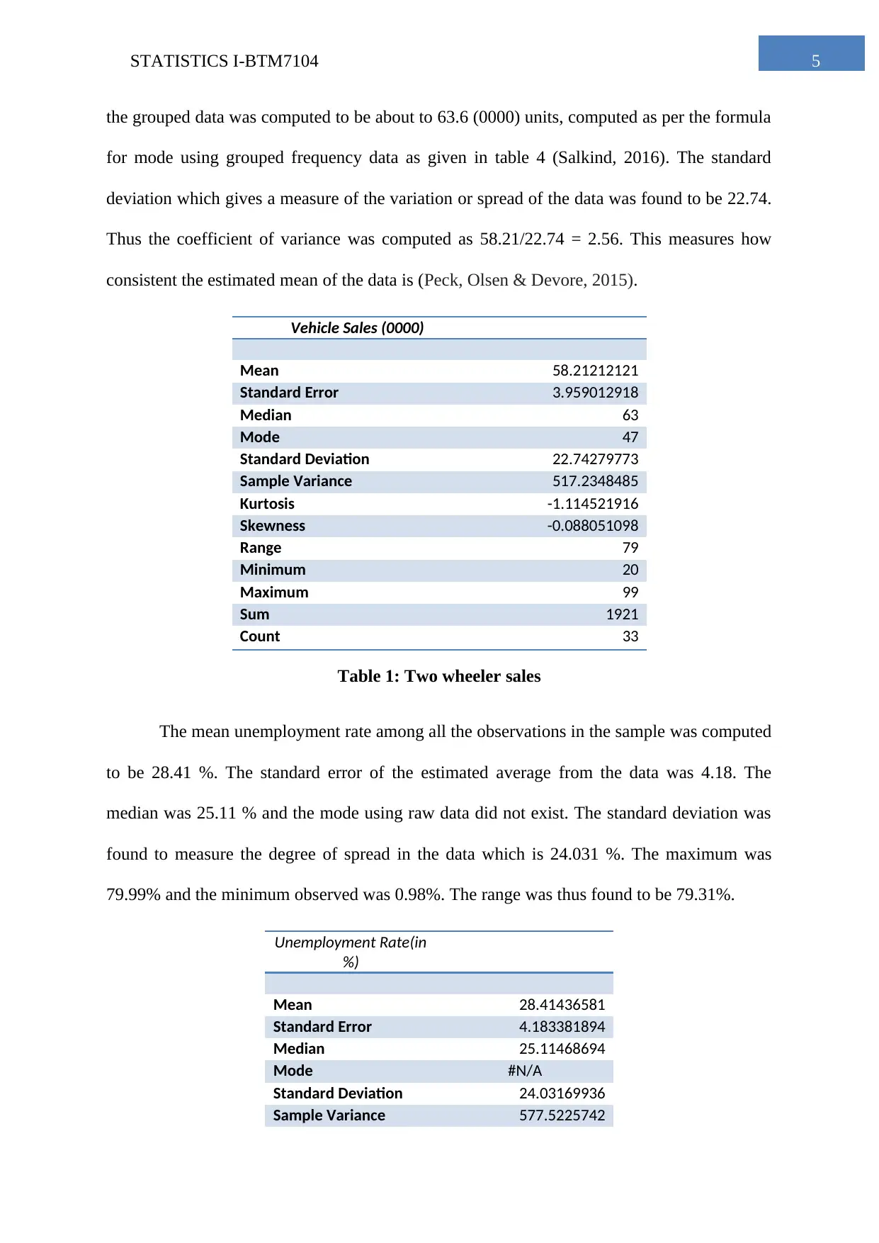
The variable vehicle sales was seen to have the mean value of 58.21 (0000) units for
the sample of data. The standard error of the estimated average was found to be 3.95. The
median was 63, that is, 50 percent of the values were less than 63 (0000) units. The mode or
the value of maximum sales was found to be 47. However since the data is raw but the
variable is a continuous variable, this is not a suitable estimate of the mode (Peck, Olsen &
Devore, 2015). The frequency distribution was referred to identify the modal class. The
modal class was found to be the interval 60 (0000) units to 69 (0000) units. The mode from
Variables and Data Description
The study defined three variables of interest relating to the two wheeled automobile
sales of a fictional country, its GDP and its rate of unemployment. The data consists of 33
observations, drawn independently under premise of simple random sampling without regard
to time. The data is hence not a time series data, ordered as per time unit. It is merely a
collection of observed sales and the corresponding GDP growth rate and unemployment rate
at the same point of time. The data is wholly defined on an interval scale. The variable sale is
recorded in 10,000 units. The variable, GDP growth rate and unemployment rates are taken
as percentages and are therefore free of units.
The dependent variable in this study is the sales volume of the two wheeler vehicles
(in 10000 units). There are two independent variables that are considered, which are the GDP
growth rate and the unemployment rate. A key assumption made while planning to design
and selecting the variables is that the dependent variable is linearly related with the
independent variables. Yet another assumption is that the two independent variables are
actually independent of each other.
Descriptive analysis
The variable vehicle sales was seen to have the mean value of 58.21 (0000) units for
the sample of data. The standard error of the estimated average was found to be 3.95. The
median was 63, that is, 50 percent of the values were less than 63 (0000) units. The mode or
the value of maximum sales was found to be 47. However since the data is raw but the
variable is a continuous variable, this is not a suitable estimate of the mode (Peck, Olsen &
Devore, 2015). The frequency distribution was referred to identify the modal class. The
modal class was found to be the interval 60 (0000) units to 69 (0000) units. The mode from
5STATISTICS I-BTM7104
the grouped data was computed to be about to 63.6 (0000) units, computed as per the formula
for mode using grouped frequency data as given in table 4 (Salkind, 2016). The standard
deviation which gives a measure of the variation or spread of the data was found to be 22.74.
Thus the coefficient of variance was computed as 58.21/22.74 = 2.56. This measures how
consistent the estimated mean of the data is (Peck, Olsen & Devore, 2015).
Vehicle Sales (0000)
Mean 58.21212121
Standard Error 3.959012918
Median 63
Mode 47
Standard Deviation 22.74279773
Sample Variance 517.2348485
Kurtosis -1.114521916
Skewness -0.088051098
Range 79
Minimum 20
Maximum 99
Sum 1921
Count 33
Table 1: Two wheeler sales
The mean unemployment rate among all the observations in the sample was computed
to be 28.41 %. The standard error of the estimated average from the data was 4.18. The
median was 25.11 % and the mode using raw data did not exist. The standard deviation was
found to measure the degree of spread in the data which is 24.031 %. The maximum was
79.99% and the minimum observed was 0.98%. The range was thus found to be 79.31%.
Unemployment Rate(in
%)
Mean 28.41436581
Standard Error 4.183381894
Median 25.11468694
Mode #N/A
Standard Deviation 24.03169936
Sample Variance 577.5225742
⊘ This is a preview!⊘
Do you want full access?
Subscribe today to unlock all pages.
Trusted by 1+ million students worldwide
6STATISTICS I-BTM7104
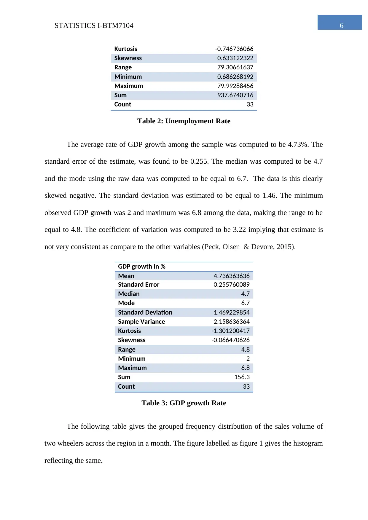
Kurtosis -0.746736066
Skewness 0.633122322
Range 79.30661637
Minimum 0.686268192
Maximum 79.99288456
Sum 937.6740716
Count 33
Table 2: Unemployment Rate
The average rate of GDP growth among the sample was computed to be 4.73%. The
standard error of the estimate, was found to be 0.255. The median was computed to be 4.7
and the mode using the raw data was computed to be equal to 6.7. The data is this clearly
skewed negative. The standard deviation was estimated to be equal to 1.46. The minimum
observed GDP growth was 2 and maximum was 6.8 among the data, making the range to be
equal to 4.8. The coefficient of variation was computed to be 3.22 implying that estimate is
not very consistent as compare to the other variables (Peck, Olsen & Devore, 2015).
GDP growth in %
Mean 4.736363636
Standard Error 0.255760089
Median 4.7
Mode 6.7
Standard Deviation 1.469229854
Sample Variance 2.158636364
Kurtosis -1.301200417
Skewness -0.066470626
Range 4.8
Minimum 2
Maximum 6.8
Sum 156.3
Count 33
Table 3: GDP growth Rate
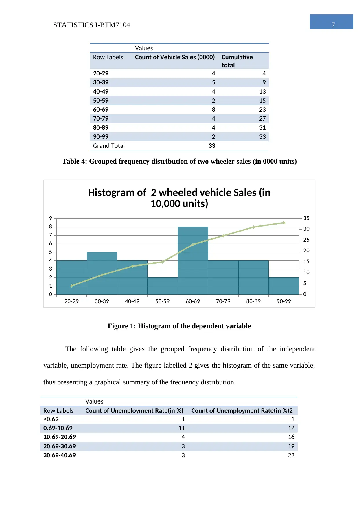
The following table gives the grouped frequency distribution of the sales volume of
two wheelers across the region in a month. The figure labelled as figure 1 gives the histogram
reflecting the same.
Kurtosis -0.746736066
Skewness 0.633122322
Range 79.30661637
Minimum 0.686268192
Maximum 79.99288456
Sum 937.6740716
Count 33
Table 2: Unemployment Rate
The average rate of GDP growth among the sample was computed to be 4.73%. The
standard error of the estimate, was found to be 0.255. The median was computed to be 4.7
and the mode using the raw data was computed to be equal to 6.7. The data is this clearly
skewed negative. The standard deviation was estimated to be equal to 1.46. The minimum
observed GDP growth was 2 and maximum was 6.8 among the data, making the range to be
equal to 4.8. The coefficient of variation was computed to be 3.22 implying that estimate is
not very consistent as compare to the other variables (Peck, Olsen & Devore, 2015).
GDP growth in %
Mean 4.736363636
Standard Error 0.255760089
Median 4.7
Mode 6.7
Standard Deviation 1.469229854
Sample Variance 2.158636364
Kurtosis -1.301200417
Skewness -0.066470626
Range 4.8
Minimum 2
Maximum 6.8
Sum 156.3
Count 33
Table 3: GDP growth Rate
The following table gives the grouped frequency distribution of the sales volume of
two wheelers across the region in a month. The figure labelled as figure 1 gives the histogram
reflecting the same.
Paraphrase This Document
Need a fresh take? Get an instant paraphrase of this document with our AI Paraphraser
7STATISTICS I-BTM7104
Values
Row Labels Count of Vehicle Sales (0000) Cumulative
total
20-29 4 4
30-39 5 9
40-49 4 13
50-59 2 15
60-69 8 23
70-79 4 27
80-89 4 31
90-99 2 33
Grand Total 33
Table 4: Grouped frequency distribution of two wheeler sales (in 0000 units)
20-29 30-39 40-49 50-59 60-69 70-79 80-89 90-99
0
1
2
3
4
5
6
7
8
9
0
5
10
15
20
25
30
35
Histogram of 2 wheeled vehicle Sales (in
10,000 units)
Figure 1: Histogram of the dependent variable
The following table gives the grouped frequency distribution of the independent
variable, unemployment rate. The figure labelled 2 gives the histogram of the same variable,
thus presenting a graphical summary of the frequency distribution.
Values
Row Labels Count of Unemployment Rate(in %) Count of Unemployment Rate(in %)2
<0.69 1 1
0.69-10.69 11 12
10.69-20.69 4 16
20.69-30.69 3 19
30.69-40.69 3 22
Values
Row Labels Count of Vehicle Sales (0000) Cumulative
total
20-29 4 4
30-39 5 9
40-49 4 13
50-59 2 15
60-69 8 23
70-79 4 27
80-89 4 31
90-99 2 33
Grand Total 33
Table 4: Grouped frequency distribution of two wheeler sales (in 0000 units)
20-29 30-39 40-49 50-59 60-69 70-79 80-89 90-99
0
1
2
3
4
5
6
7
8
9
0
5
10
15
20
25
30
35
Histogram of 2 wheeled vehicle Sales (in
10,000 units)
Figure 1: Histogram of the dependent variable
The following table gives the grouped frequency distribution of the independent
variable, unemployment rate. The figure labelled 2 gives the histogram of the same variable,
thus presenting a graphical summary of the frequency distribution.
Values
Row Labels Count of Unemployment Rate(in %) Count of Unemployment Rate(in %)2
<0.69 1 1
0.69-10.69 11 12
10.69-20.69 4 16
20.69-30.69 3 19
30.69-40.69 3 22
8STATISTICS I-BTM7104
40.69-50.69 4 26
50.69-60.69 4 30
60.69-70.69 1 31
70.69-80.69 1 32
>80.69 1 33
Grand Total 33
Table 5: Grouped frequency distribution of unemployment rates
<0.69 0.69-
10.69 10.69-
20.69 20.69-
30.69 30.69-
40.69 40.69-
50.69 50.69-
60.69 60.69-
70.69 70.69-
80.69 >80.69
0
2
4
6
8
10
12
0
5
10
15
20
25
30
35
Histogram of unemployment rate in
percentage
Figure 2: Histogram of unemployment rate
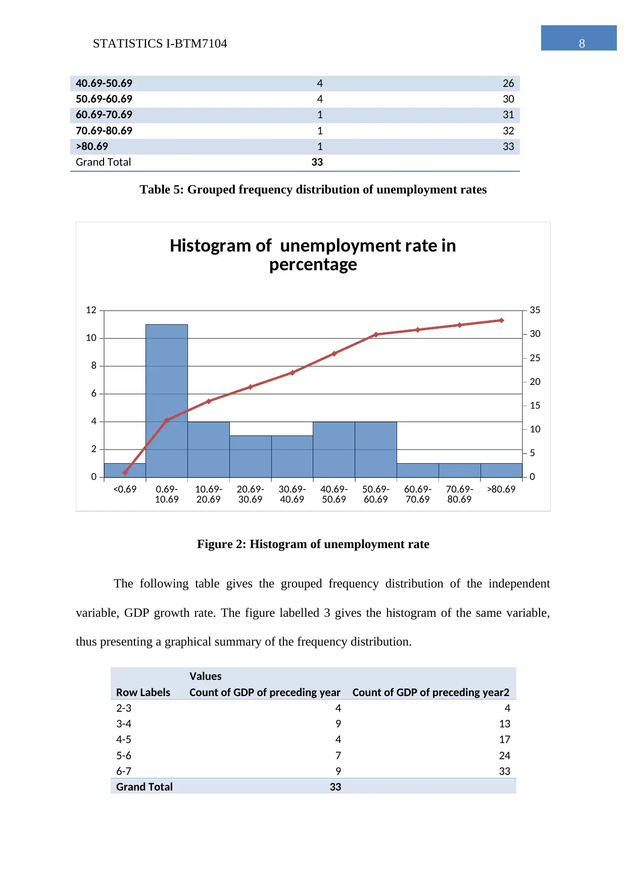
The following table gives the grouped frequency distribution of the independent
variable, GDP growth rate. The figure labelled 3 gives the histogram of the same variable,
thus presenting a graphical summary of the frequency distribution.
Values
Row Labels Count of GDP of preceding year Count of GDP of preceding year2
2-3 4 4
3-4 9 13
4-5 4 17
5-6 7 24
6-7 9 33
Grand Total 33
40.69-50.69 4 26
50.69-60.69 4 30
60.69-70.69 1 31
70.69-80.69 1 32
>80.69 1 33
Grand Total 33
Table 5: Grouped frequency distribution of unemployment rates
<0.69 0.69-
10.69 10.69-
20.69 20.69-
30.69 30.69-
40.69 40.69-
50.69 50.69-
60.69 60.69-
70.69 70.69-
80.69 >80.69
0
2
4
6
8
10
12
0
5
10
15
20
25
30
35
Histogram of unemployment rate in
percentage
Figure 2: Histogram of unemployment rate
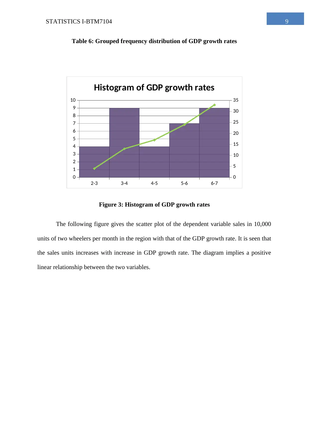
The following table gives the grouped frequency distribution of the independent
variable, GDP growth rate. The figure labelled 3 gives the histogram of the same variable,
thus presenting a graphical summary of the frequency distribution.
Values
Row Labels Count of GDP of preceding year Count of GDP of preceding year2
2-3 4 4
3-4 9 13
4-5 4 17
5-6 7 24
6-7 9 33
Grand Total 33
⊘ This is a preview!⊘
Do you want full access?
Subscribe today to unlock all pages.
Trusted by 1+ million students worldwide
9STATISTICS I-BTM7104
Table 6: Grouped frequency distribution of GDP growth rates
2-3 3-4 4-5 5-6 6-7
0
1
2
3
4
5
6
7
8
9
10
0
5
10
15
20
25
30
35
Histogram of GDP growth rates
Figure 3: Histogram of GDP growth rates
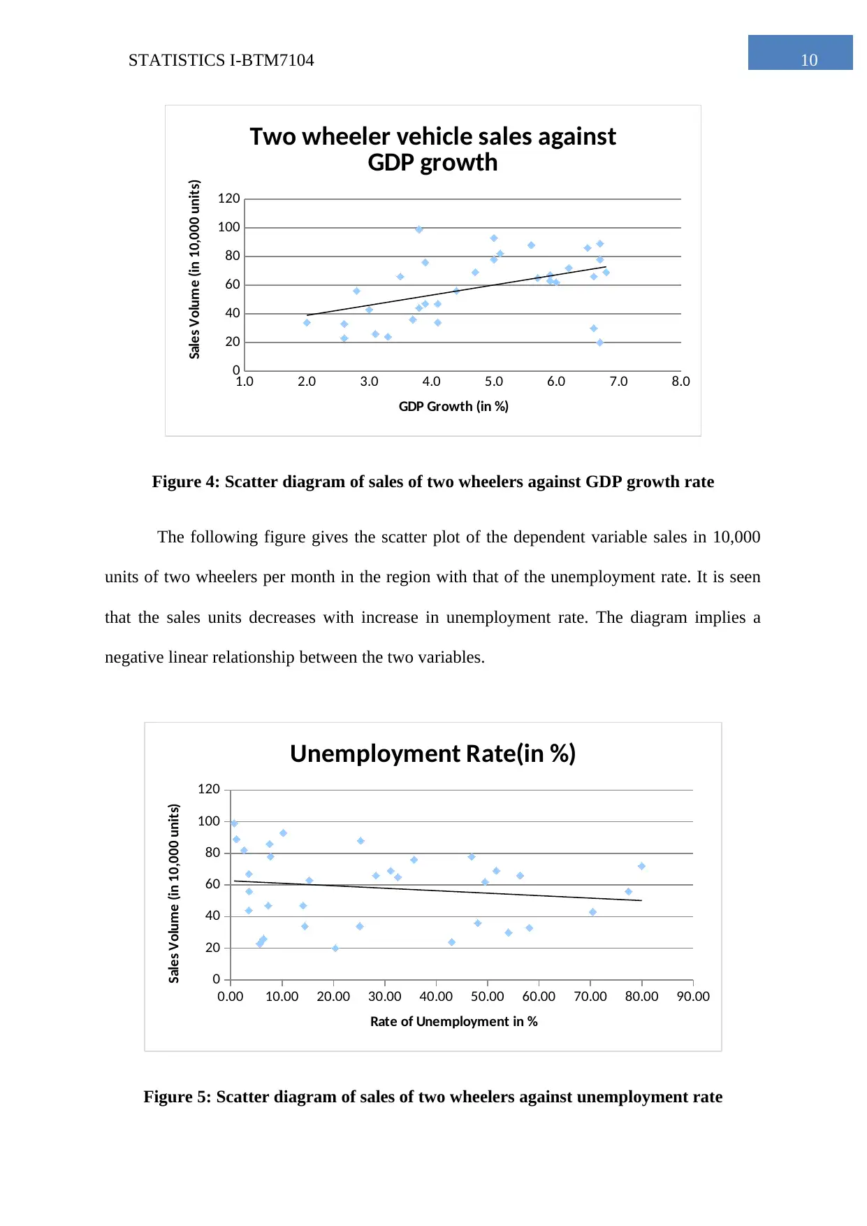
The following figure gives the scatter plot of the dependent variable sales in 10,000
units of two wheelers per month in the region with that of the GDP growth rate. It is seen that
the sales units increases with increase in GDP growth rate. The diagram implies a positive
linear relationship between the two variables.
Table 6: Grouped frequency distribution of GDP growth rates
2-3 3-4 4-5 5-6 6-7
0
1
2
3
4
5
6
7
8
9
10
0
5
10
15
20
25
30
35
Histogram of GDP growth rates
Figure 3: Histogram of GDP growth rates
The following figure gives the scatter plot of the dependent variable sales in 10,000
units of two wheelers per month in the region with that of the GDP growth rate. It is seen that
the sales units increases with increase in GDP growth rate. The diagram implies a positive
linear relationship between the two variables.
Paraphrase This Document
Need a fresh take? Get an instant paraphrase of this document with our AI Paraphraser
10STATISTICS I-BTM7104
1.0 2.0 3.0 4.0 5.0 6.0 7.0 8.0
0
20
40
60
80
100
120
Two wheeler vehicle sales against
GDP growth
GDP Growth (in %)
Sales Volume (in 10,000 units)
Figure 4: Scatter diagram of sales of two wheelers against GDP growth rate
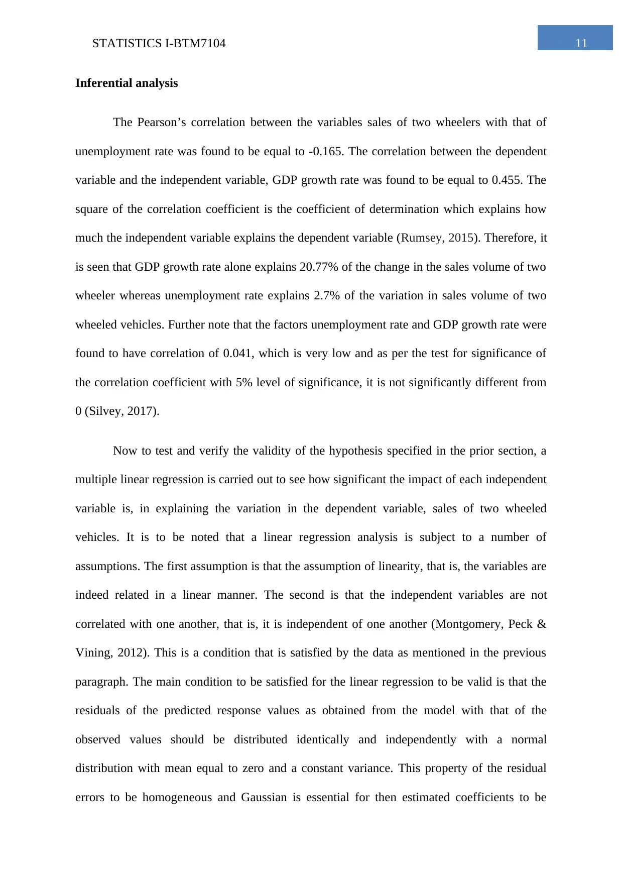
The following figure gives the scatter plot of the dependent variable sales in 10,000
units of two wheelers per month in the region with that of the unemployment rate. It is seen
that the sales units decreases with increase in unemployment rate. The diagram implies a
negative linear relationship between the two variables.
0.00 10.00 20.00 30.00 40.00 50.00 60.00 70.00 80.00 90.00
0
20
40
60
80
100
120
Unemployment Rate(in %)
Rate of Unemployment in %
Sales Volume (in 10,000 units)
Figure 5: Scatter diagram of sales of two wheelers against unemployment rate
1.0 2.0 3.0 4.0 5.0 6.0 7.0 8.0
0
20
40
60
80
100
120
Two wheeler vehicle sales against
GDP growth
GDP Growth (in %)
Sales Volume (in 10,000 units)
Figure 4: Scatter diagram of sales of two wheelers against GDP growth rate
The following figure gives the scatter plot of the dependent variable sales in 10,000
units of two wheelers per month in the region with that of the unemployment rate. It is seen
that the sales units decreases with increase in unemployment rate. The diagram implies a
negative linear relationship between the two variables.
0.00 10.00 20.00 30.00 40.00 50.00 60.00 70.00 80.00 90.00
0
20
40
60
80
100
120
Unemployment Rate(in %)
Rate of Unemployment in %
Sales Volume (in 10,000 units)
Figure 5: Scatter diagram of sales of two wheelers against unemployment rate
11STATISTICS I-BTM7104
Inferential analysis
The Pearson’s correlation between the variables sales of two wheelers with that of
unemployment rate was found to be equal to -0.165. The correlation between the dependent
variable and the independent variable, GDP growth rate was found to be equal to 0.455. The
square of the correlation coefficient is the coefficient of determination which explains how
much the independent variable explains the dependent variable (Rumsey, 2015). Therefore, it
is seen that GDP growth rate alone explains 20.77% of the change in the sales volume of two
wheeler whereas unemployment rate explains 2.7% of the variation in sales volume of two
wheeled vehicles. Further note that the factors unemployment rate and GDP growth rate were
found to have correlation of 0.041, which is very low and as per the test for significance of
the correlation coefficient with 5% level of significance, it is not significantly different from
0 (Silvey, 2017).
Now to test and verify the validity of the hypothesis specified in the prior section, a
multiple linear regression is carried out to see how significant the impact of each independent
variable is, in explaining the variation in the dependent variable, sales of two wheeled
vehicles. It is to be noted that a linear regression analysis is subject to a number of
assumptions. The first assumption is that the assumption of linearity, that is, the variables are
indeed related in a linear manner. The second is that the independent variables are not
correlated with one another, that is, it is independent of one another (Montgomery, Peck &
Vining, 2012). This is a condition that is satisfied by the data as mentioned in the previous
paragraph. The main condition to be satisfied for the linear regression to be valid is that the
residuals of the predicted response values as obtained from the model with that of the
observed values should be distributed identically and independently with a normal
distribution with mean equal to zero and a constant variance. This property of the residual
errors to be homogeneous and Gaussian is essential for then estimated coefficients to be
⊘ This is a preview!⊘
Do you want full access?
Subscribe today to unlock all pages.
Trusted by 1+ million students worldwide
1 out of 20


Your All-in-One AI-Powered Toolkit for Academic Success.
+13062052269
info@desklib.com
Available 24*7 on WhatsApp / Email
![[object Object]](/_next/static/media/star-bottom.7253800d.svg)
Unlock your academic potential
Copyright © 2020–2026 A2Z Services. All Rights Reserved. Developed and managed by ZUCOL.