University of Florida STA 2023 Midterm 2: Citrus Production Analysis
VerifiedAdded on 2022/07/28
|9
|2194
|32
Homework Assignment
AI Summary
This document presents a solved midterm exam from a statistics course, likely at the University of Florida (UF), focusing on the statistical analysis of citrus production data. The exam consists of 20 multiple-choice questions, covering a range of statistical concepts including hypothesis testing, confidence intervals, regression analysis (both simple and multiple), and ANOVA. The questions utilize provided exhibits with data related to citrus greening, production, prices, and insecticide application. Students are expected to interpret data, perform calculations (critical values, test statistics, p-values), and draw conclusions based on the statistical analyses. The exam assesses the student's ability to apply statistical methods to real-world scenarios and interpret the results in the context of the given data, such as determining the significance of relationships between variables like price, production, and the impact of citrus greening.
Midterm 2
Please:
Sign your name below and write your name in print here: ______________________ ID:
________________
Read each question carefully before choosing your answer.
Please circle the correct answer and write the letter on the cover page of this exam.
Partial credit may be awarded in the event that you respond incorrectly but it is clear
that you understand the topic.
There are 20 total multiple choice questions in this exam worth 5 points each
This is an open-book, open-note exam but it is an individual assessment and all work is
expected to be independent (no sharing with friends, having someone take it for you,
etc.) You should be aware of the UF honor code by now, but if you need a reminder,
please see the following link: https://sccr.dso.ufl.edu/policies/student-honor-code-
student-conduct-code/
Do not hesitate to ask me questions regarding this exam (mistisharp@ufl.edu). I will
respond as quickly as a can although I will not be answering questions after 5 pm on
Monday.
A scanned pdf of this entire assignment needs to be uploaded on the assignment in e-
learning BEFORE midnight on Monday, April 20th. You can use a printer to scan or
there are apps on your phone (such as camscanner) that will convert images to pdfs. If
you do not have printing resources, you may type your responses and take pictures of
your handwritten work to include in addition.
Question:
1 C 14 A
2 B 15 D
3 A 16 C
4 D 17 B
5 D 18 B
6 A 19 C
7 D 20 C
8 A Bonus
9 B
10 A
11 D
12 A
13 B
SCOR
E:
(out of
100)
VA 1
Paraphrase This Document
Need a fresh take? Get an instant paraphrase of this document with our AI Paraphraser

Name: ______________________________ UF Honor Pledge: We, the members of the University of
Florida Community, pledge to hold ourselves and our peers to the highest standards of honesty
and integrity.
VA 2
Florida Community, pledge to hold ourselves and our peers to the highest standards of honesty
and integrity.
VA 2
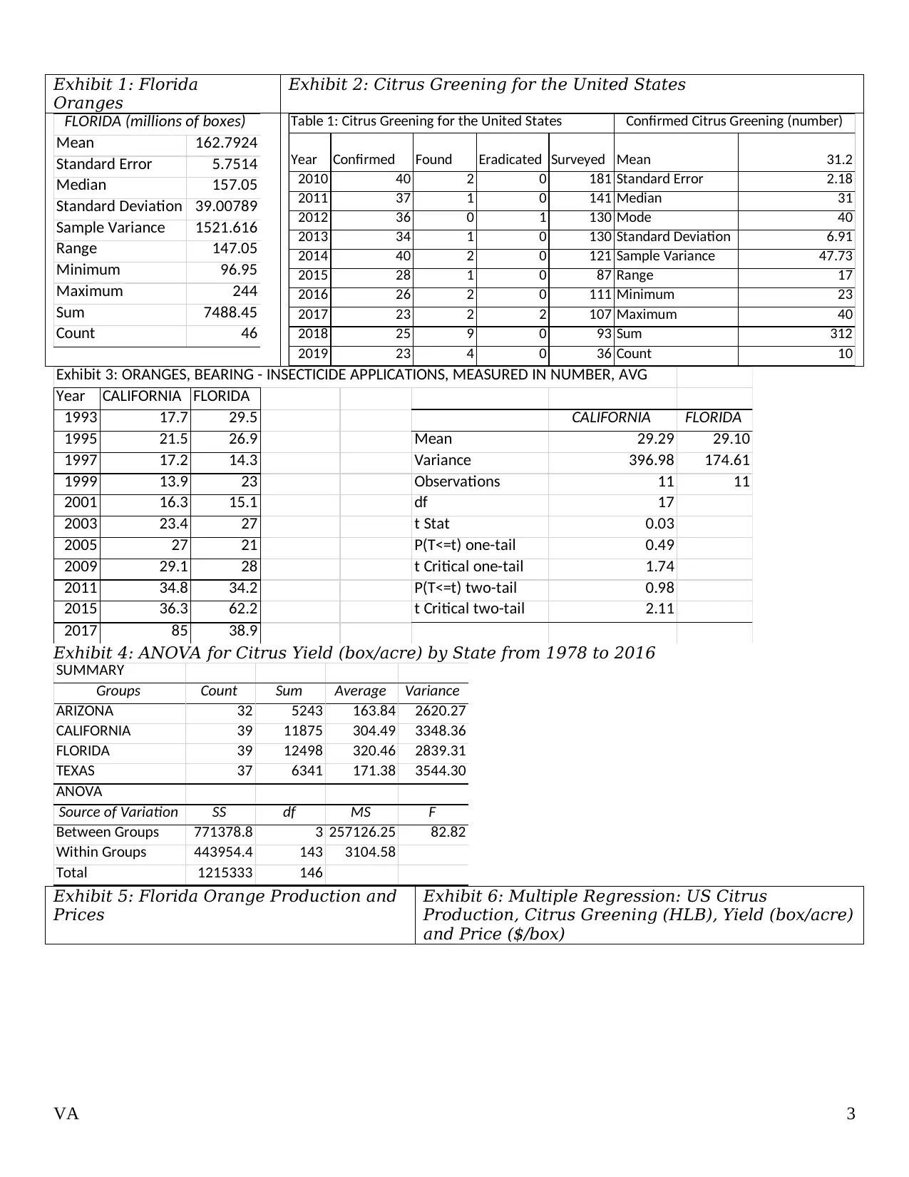
Exhibit 1: Florida
Oranges
Exhibit 2: Citrus Greening for the United States
Mean 162.7924
Standard Error 5.7514
Median 157.05
Standard Deviation 39.00789
Sample Variance 1521.616
Range 147.05
Minimum 96.95
Maximum 244
Sum 7488.45
Count 46
FLORIDA (millions of boxes) Table 1: Citrus Greening for the United States
Year Confirmed Found Eradicated Surveyed Mean 31.2
2010 40 2 0 181 Standard Error 2.18
2011 37 1 0 141 Median 31
2012 36 0 1 130 Mode 40
2013 34 1 0 130 Standard Deviation 6.91
2014 40 2 0 121 Sample Variance 47.73
2015 28 1 0 87 Range 17
2016 26 2 0 111 Minimum 23
2017 23 2 2 107 Maximum 40
2018 25 9 0 93 Sum 312
2019 23 4 0 36 Count 10
Confirmed Citrus Greening (number)
Exhibit 3: ORANGES, BEARING - INSECTICIDE APPLICATIONS, MEASURED IN NUMBER, AVG
Year CALIFORNIA FLORIDA
1993 17.7 29.5 CALIFORNIA FLORIDA
1995 21.5 26.9 Mean 29.29 29.10
1997 17.2 14.3 Variance 396.98 174.61
1999 13.9 23 Observations 11 11
2001 16.3 15.1 df 17
2003 23.4 27 t Stat 0.03
2005 27 21 P(T<=t) one-tail 0.49
2009 29.1 28 t Critical one-tail 1.74
2011 34.8 34.2 P(T<=t) two-tail 0.98
2015 36.3 62.2 t Critical two-tail 2.11
2017 85 38.9
322.2 320.1Exhibit 4: ANOVA for Citrus Yield (box/acre) by State from 1978 to 2016
SUMMARY
Groups Count Sum Average Variance
ARIZONA 32 5243 163.84 2620.27
CALIFORNIA 39 11875 304.49 3348.36
FLORIDA 39 12498 320.46 2839.31
TEXAS 37 6341 171.38 3544.30
ANOVA
Source of Variation SS df MS F
Between Groups 771378.8 3 257126.25 82.82
Within Groups 443954.4 143 3104.58
Total 1215333 146
Exhibit 5: Florida Orange Production and
Prices
Exhibit 6: Multiple Regression: US Citrus
Production, Citrus Greening (HLB), Yield (box/acre)
and Price ($/box)
VA 3
⊘ This is a preview!⊘
Do you want full access?
Subscribe today to unlock all pages.
Trusted by 1+ million students worldwide
2 3 4 5 6 7 8 9 10 11
90
110
130
150
170
190
210
230
250
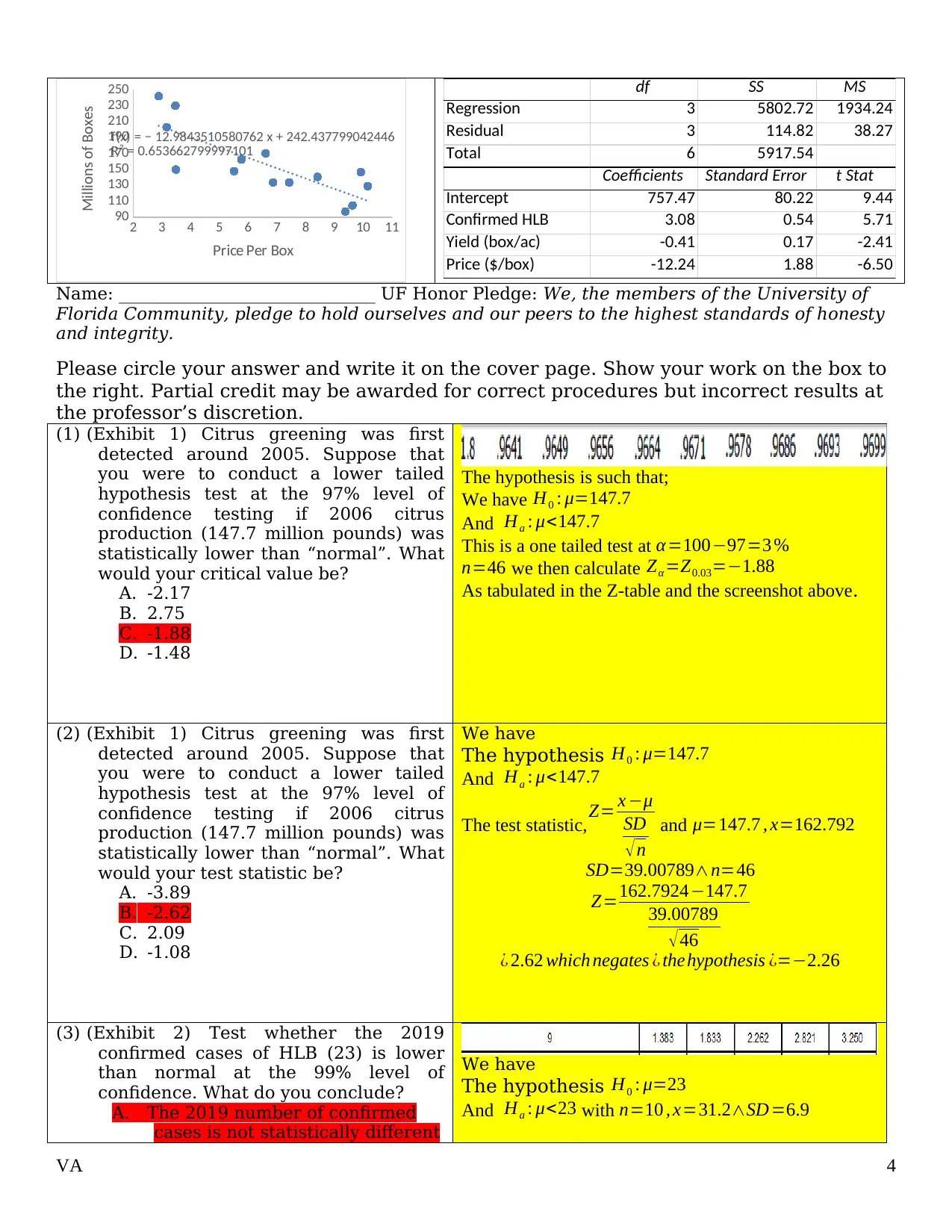
f(x) = − 12.9843510580762 x + 242.437799042446
R² = 0.653662799997101
Price Per Box
Millions of Boxes df SS MS
Regression 3 5802.72 1934.24
Residual 3 114.82 38.27
Total 6 5917.54
Coefficients Standard Error t Stat
Intercept 757.47 80.22 9.44
Confirmed HLB 3.08 0.54 5.71
Yield (box/ac) -0.41 0.17 -2.41
Price ($/box) -12.24 1.88 -6.50
Name: ______________________________ UF Honor Pledge: We, the members of the University of
Florida Community, pledge to hold ourselves and our peers to the highest standards of honesty
and integrity.
Please circle your answer and write it on the cover page. Show your work on the box to
the right. Partial credit may be awarded for correct procedures but incorrect results at
the professor’s discretion.
(1) (Exhibit 1) Citrus greening was first
detected around 2005. Suppose that
you were to conduct a lower tailed
hypothesis test at the 97% level of
confidence testing if 2006 citrus
production (147.7 million pounds) was
statistically lower than “normal”. What
would your critical value be?
A. -2.17
B. 2.75
C. -1.88
D. -1.48
The hypothesis is such that;
We have H0 : μ=147.7
And Ha : μ<147.7
This is a one tailed test at α=100−97=3 %
n=46 we then calculate Zα=Z0.03=−1.88
As tabulated in the Z-table and the screenshot above.
(2) (Exhibit 1) Citrus greening was first
detected around 2005. Suppose that
you were to conduct a lower tailed
hypothesis test at the 97% level of
confidence testing if 2006 citrus
production (147.7 million pounds) was
statistically lower than “normal”. What
would your test statistic be?
A. -3.89
B. -2.62
C. 2.09
D. -1.08
We have
The hypothesis H0 : μ=147.7
And Ha : μ<147.7
The test statistic, Z= x −μ
SD
√ n
and μ=147.7 , x=162.792
SD=39.00789∧n=46
Z=162.7924−147.7
39.00789
√46
¿ 2.62 which negates ¿ thehypothesis ¿=−2.26
(3) (Exhibit 2) Test whether the 2019
confirmed cases of HLB (23) is lower
than normal at the 99% level of
confidence. What do you conclude?
A. The 2019 number of confirmed
cases is not statistically different
We have
The hypothesis H0 : μ=23
And Ha : μ<23 with n=10 , x=31.2∧SD =6.9
VA 4
90
110
130
150
170
190
210
230
250
f(x) = − 12.9843510580762 x + 242.437799042446
R² = 0.653662799997101
Price Per Box
Millions of Boxes df SS MS
Regression 3 5802.72 1934.24
Residual 3 114.82 38.27
Total 6 5917.54
Coefficients Standard Error t Stat
Intercept 757.47 80.22 9.44
Confirmed HLB 3.08 0.54 5.71
Yield (box/ac) -0.41 0.17 -2.41
Price ($/box) -12.24 1.88 -6.50
Name: ______________________________ UF Honor Pledge: We, the members of the University of
Florida Community, pledge to hold ourselves and our peers to the highest standards of honesty
and integrity.
Please circle your answer and write it on the cover page. Show your work on the box to
the right. Partial credit may be awarded for correct procedures but incorrect results at
the professor’s discretion.
(1) (Exhibit 1) Citrus greening was first
detected around 2005. Suppose that
you were to conduct a lower tailed
hypothesis test at the 97% level of
confidence testing if 2006 citrus
production (147.7 million pounds) was
statistically lower than “normal”. What
would your critical value be?
A. -2.17
B. 2.75
C. -1.88
D. -1.48
The hypothesis is such that;
We have H0 : μ=147.7
And Ha : μ<147.7
This is a one tailed test at α=100−97=3 %
n=46 we then calculate Zα=Z0.03=−1.88
As tabulated in the Z-table and the screenshot above.
(2) (Exhibit 1) Citrus greening was first
detected around 2005. Suppose that
you were to conduct a lower tailed
hypothesis test at the 97% level of
confidence testing if 2006 citrus
production (147.7 million pounds) was
statistically lower than “normal”. What
would your test statistic be?
A. -3.89
B. -2.62
C. 2.09
D. -1.08
We have
The hypothesis H0 : μ=147.7
And Ha : μ<147.7
The test statistic, Z= x −μ
SD
√ n
and μ=147.7 , x=162.792
SD=39.00789∧n=46
Z=162.7924−147.7
39.00789
√46
¿ 2.62 which negates ¿ thehypothesis ¿=−2.26
(3) (Exhibit 2) Test whether the 2019
confirmed cases of HLB (23) is lower
than normal at the 99% level of
confidence. What do you conclude?
A. The 2019 number of confirmed
cases is not statistically different
We have
The hypothesis H0 : μ=23
And Ha : μ<23 with n=10 , x=31.2∧SD =6.9
VA 4
Paraphrase This Document
Need a fresh take? Get an instant paraphrase of this document with our AI Paraphraser
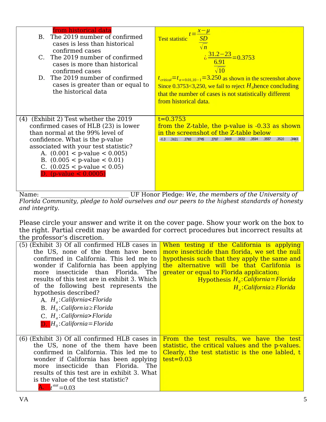
from historical data
B. The 2019 number of confirmed
cases is less than historical
confirmed cases
C. The 2019 number of confirmed
cases is more than historical
confirmed cases
D. The 2019 number of confirmed
cases is greater than or equal to
the historical data
Test statistic t= x−μ
SD
√ n
¿ 31.2−23
6.91
√10
=0.3753
tcritical=tα =0.01,10−1=3.250 as shown in the screenshot above
Since 0.3753<3,250, we fail to reject H0hence concluding
that the number of cases is not statistically different
from historical data.
(4) (Exhibit 2) Test whether the 2019
confirmed cases of HLB (23) is lower
than normal at the 99% level of
confidence. What is the p-value
associated with your test statistic?
A. (0.001 < p-value < 0.005)
B. (0.005 < p-value < 0.01)
C. (0.025 < p-value < 0.05)
D. (p-value < 0.0005)
t=0.3753
from the Z-table, the p-value is -0.33 as shown
in the screenshot of the Z-table below
Name: ______________________________ UF Honor Pledge: We, the members of the University of
Florida Community, pledge to hold ourselves and our peers to the highest standards of honesty
and integrity.
Please circle your answer and write it on the cover page. Show your work on the box to
the right. Partial credit may be awarded for correct procedures but incorrect results at
the professor’s discretion.
(5) (Exhibit 3) Of all confirmed HLB cases in
the US, none of the them have been
confirmed in California. This led me to
wonder if California has been applying
more insecticide than Florida. The
results of this test are in exhibit 3. Which
of the following best represents the
hypothesis described?
A. Ha :California<Florida
B. H0 :Californ ia≥ Florida
C. Ha :California>Florida
D. H0 :California=Florida
When testing if the California is applying
more insecticide than florida, we set the null
hypothesis such that they apply the same and
the alternative will be that Carlifonia is
greater or equal to Florida application;
Hypothesis H0 :California=Florida
Ha :California≥ Florida
(6) (Exhibit 3) Of all confirmed HLB cases in
the US, none of the them have been
confirmed in California. This led me to
wonder if California has been applying
more insecticide than Florida. The
results of this test are in exhibit 3. What
is the value of the test statistic?
A. tstat =0.03
From the test results, we have the test
statistic, the critical values and the p-values.
Clearly, the test statistic is the one labled, t
test=0.03
VA 5
B. tstat =0.49
C. tstat =1.74
D. tstat =−2.11
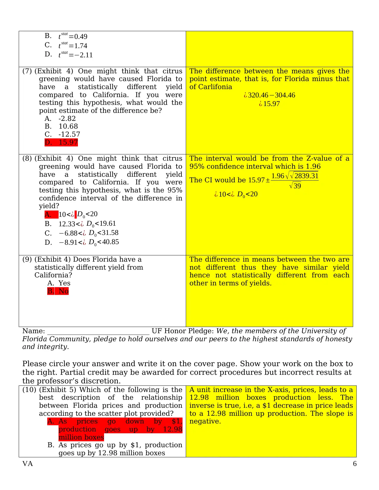
(7) (Exhibit 4) One might think that citrus
greening would have caused Florida to
have a statistically different yield
compared to California. If you were
testing this hypothesis, what would the
point estimate of the difference be?
A. -2.82
B. 10.68
C. -12.57
D. 15.97
The difference between the means gives the
point estimate, that is, for Florida minus that
of Carlifonia
¿ 320.46−304.46
¿ 15.97
(8) (Exhibit 4) One might think that citrus
greening would have caused Florida to
have a statistically different yield
compared to California. If you were
testing this hypothesis, what is the 95%
confidence interval of the difference in
yield?
A. 10<¿ D0 <20
B. 12.33<¿ D0 <19.61
C. −6.88<¿ D0 <31.58
D. −8.91<¿ D0 < 40.85
The interval would be from the Z-value of a
95% confidence interval which is 1.96
The CI would be 15.97 ± 1.96 √ √2839.31
√39
¿ 10<¿ D0 <20
(9) (Exhibit 4) Does Florida have a
statistically different yield from
California?
A. Yes
B. No
The difference in means between the two are
not different thus they have similar yield
hence not statistically different from each
other in terms of yields.
Name: ______________________________ UF Honor Pledge: We, the members of the University of
Florida Community, pledge to hold ourselves and our peers to the highest standards of honesty
and integrity.
Please circle your answer and write it on the cover page. Show your work on the box to
the right. Partial credit may be awarded for correct procedures but incorrect results at
the professor’s discretion.
(10) (Exhibit 5) Which of the following is the
best description of the relationship
between Florida prices and production
according to the scatter plot provided?
A. As prices go down by $1,
production goes up by 12.98
million boxes
B. As prices go up by $1, production
goes up by 12.98 million boxes
A unit increase in the X-axis, prices, leads to a
12.98 million boxes production less. The
inverse is true, i.e, a $1 decrease in price leads
to a 12.98 million up production. The slope is
negative.
VA 6
C. tstat =1.74
D. tstat =−2.11
(7) (Exhibit 4) One might think that citrus
greening would have caused Florida to
have a statistically different yield
compared to California. If you were
testing this hypothesis, what would the
point estimate of the difference be?
A. -2.82
B. 10.68
C. -12.57
D. 15.97
The difference between the means gives the
point estimate, that is, for Florida minus that
of Carlifonia
¿ 320.46−304.46
¿ 15.97
(8) (Exhibit 4) One might think that citrus
greening would have caused Florida to
have a statistically different yield
compared to California. If you were
testing this hypothesis, what is the 95%
confidence interval of the difference in
yield?
A. 10<¿ D0 <20
B. 12.33<¿ D0 <19.61
C. −6.88<¿ D0 <31.58
D. −8.91<¿ D0 < 40.85
The interval would be from the Z-value of a
95% confidence interval which is 1.96
The CI would be 15.97 ± 1.96 √ √2839.31
√39
¿ 10<¿ D0 <20
(9) (Exhibit 4) Does Florida have a
statistically different yield from
California?
A. Yes
B. No
The difference in means between the two are
not different thus they have similar yield
hence not statistically different from each
other in terms of yields.
Name: ______________________________ UF Honor Pledge: We, the members of the University of
Florida Community, pledge to hold ourselves and our peers to the highest standards of honesty
and integrity.
Please circle your answer and write it on the cover page. Show your work on the box to
the right. Partial credit may be awarded for correct procedures but incorrect results at
the professor’s discretion.
(10) (Exhibit 5) Which of the following is the
best description of the relationship
between Florida prices and production
according to the scatter plot provided?
A. As prices go down by $1,
production goes up by 12.98
million boxes
B. As prices go up by $1, production
goes up by 12.98 million boxes
A unit increase in the X-axis, prices, leads to a
12.98 million boxes production less. The
inverse is true, i.e, a $1 decrease in price leads
to a 12.98 million up production. The slope is
negative.
VA 6
⊘ This is a preview!⊘
Do you want full access?
Subscribe today to unlock all pages.
Trusted by 1+ million students worldwide
C. As production goes down by 1
million boxes, prices decrease by
$12.98
D. As production goes up by 1 million
boxes, prices go down by $12.98
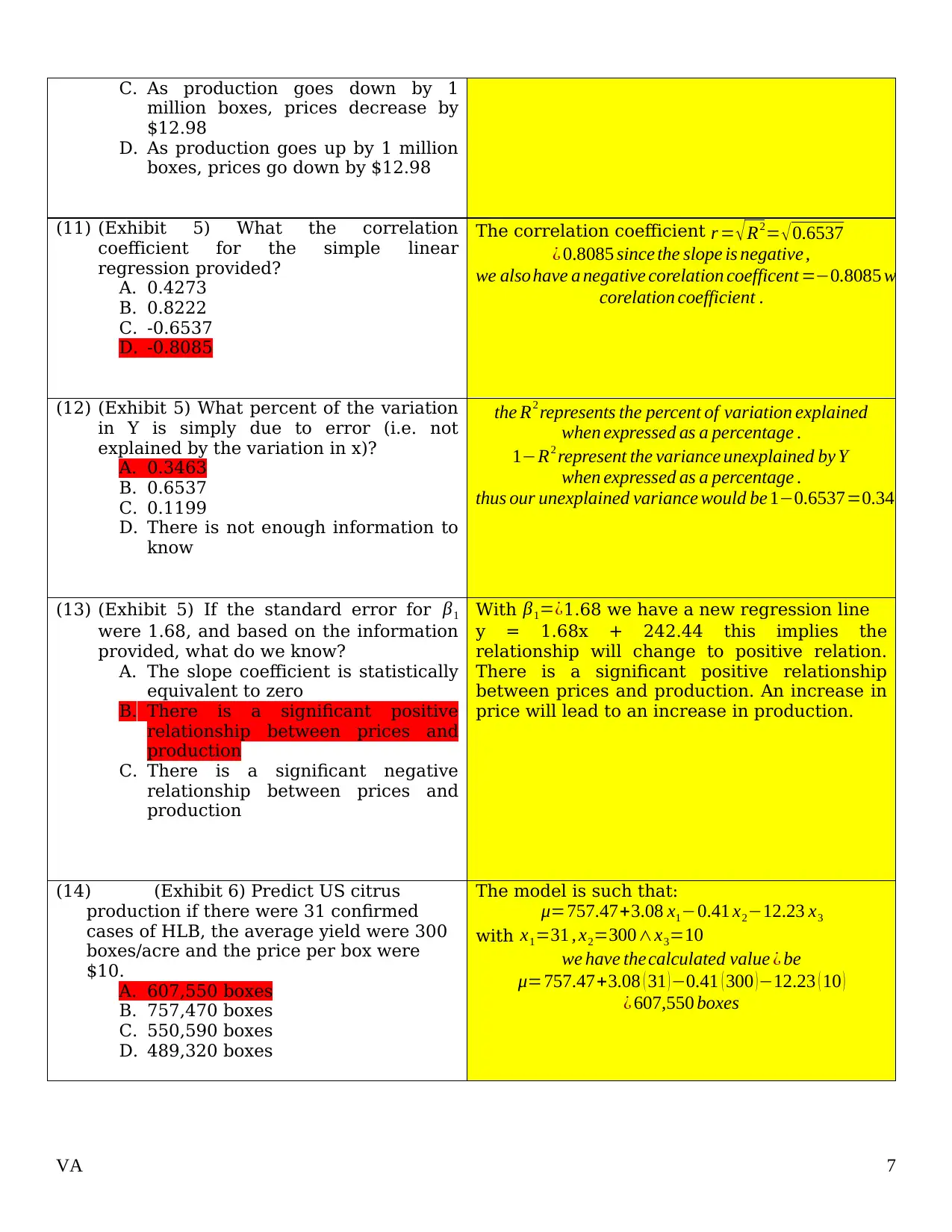
(11) (Exhibit 5) What the correlation
coefficient for the simple linear
regression provided?
A. 0.4273
B. 0.8222
C. -0.6537
D. -0.8085
The correlation coefficient r = √R2= √0.6537
¿ 0.8085 since the slope is negative ,
we alsohave a negative corelation coefficent =−0.8085 which sho
corelation coefficient .
(12) (Exhibit 5) What percent of the variation
in Y is simply due to error (i.e. not
explained by the variation in x)?
A. 0.3463
B. 0.6537
C. 0.1199
D. There is not enough information to
know
the R2 represents the percent of variation explained
when expressed as a percentage .
1−R2 represent the variance unexplained by Y
when expressed as a percentage .
thus our unexplained variance would be 1−0.6537=0.3463
(13) (Exhibit 5) If the standard error for β1
were 1.68, and based on the information
provided, what do we know?
A. The slope coefficient is statistically
equivalent to zero
B. There is a significant positive
relationship between prices and
production
C. There is a significant negative
relationship between prices and
production
With β1=¿1.68 we have a new regression line
y = 1.68x + 242.44 this implies the
relationship will change to positive relation.
There is a significant positive relationship
between prices and production. An increase in
price will lead to an increase in production.
(14) (Exhibit 6) Predict US citrus
production if there were 31 confirmed
cases of HLB, the average yield were 300
boxes/acre and the price per box were
$10.
A. 607,550 boxes
B. 757,470 boxes
C. 550,590 boxes
D. 489,320 boxes
The model is such that:
μ=757.47+3.08 x1−0.41 x2−12.23 x3
with x1=31 , x2=300∧x3=10
we have thecalculated value ¿ be
μ=757.47+3.08 ( 31 )−0.41 ( 300 )−12.23 ( 10 )
¿ 607,550 boxes
VA 7
million boxes, prices decrease by
$12.98
D. As production goes up by 1 million
boxes, prices go down by $12.98
(11) (Exhibit 5) What the correlation
coefficient for the simple linear
regression provided?
A. 0.4273
B. 0.8222
C. -0.6537
D. -0.8085
The correlation coefficient r = √R2= √0.6537
¿ 0.8085 since the slope is negative ,
we alsohave a negative corelation coefficent =−0.8085 which sho
corelation coefficient .
(12) (Exhibit 5) What percent of the variation
in Y is simply due to error (i.e. not
explained by the variation in x)?
A. 0.3463
B. 0.6537
C. 0.1199
D. There is not enough information to
know
the R2 represents the percent of variation explained
when expressed as a percentage .
1−R2 represent the variance unexplained by Y
when expressed as a percentage .
thus our unexplained variance would be 1−0.6537=0.3463
(13) (Exhibit 5) If the standard error for β1
were 1.68, and based on the information
provided, what do we know?
A. The slope coefficient is statistically
equivalent to zero
B. There is a significant positive
relationship between prices and
production
C. There is a significant negative
relationship between prices and
production
With β1=¿1.68 we have a new regression line
y = 1.68x + 242.44 this implies the
relationship will change to positive relation.
There is a significant positive relationship
between prices and production. An increase in
price will lead to an increase in production.
(14) (Exhibit 6) Predict US citrus
production if there were 31 confirmed
cases of HLB, the average yield were 300
boxes/acre and the price per box were
$10.
A. 607,550 boxes
B. 757,470 boxes
C. 550,590 boxes
D. 489,320 boxes
The model is such that:
μ=757.47+3.08 x1−0.41 x2−12.23 x3
with x1=31 , x2=300∧x3=10
we have thecalculated value ¿ be
μ=757.47+3.08 ( 31 )−0.41 ( 300 )−12.23 ( 10 )
¿ 607,550 boxes
VA 7
Paraphrase This Document
Need a fresh take? Get an instant paraphrase of this document with our AI Paraphraser
Name: ______________________________ UF Honor Pledge: We, the members of the University of
Florida Community, pledge to hold ourselves and our peers to the highest standards of honesty
and integrity.
Please circle your answer and write it on the cover page. Show your work on the box to
the right. Partial credit may be awarded for correct procedures but incorrect results at
the professor’s discretion.
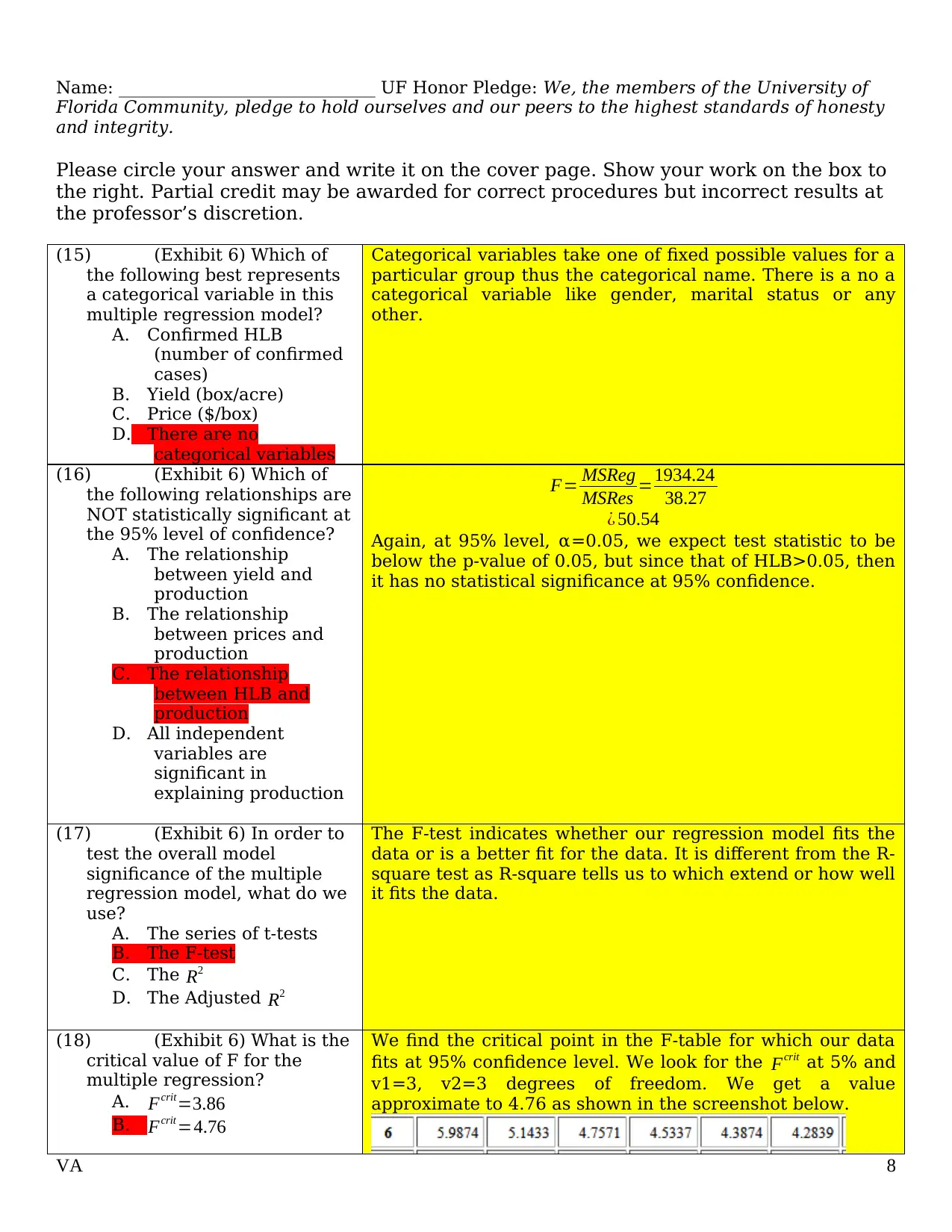
(15) (Exhibit 6) Which of
the following best represents
a categorical variable in this
multiple regression model?
A. Confirmed HLB
(number of confirmed
cases)
B. Yield (box/acre)
C. Price ($/box)
D. There are no
categorical variables
Categorical variables take one of fixed possible values for a
particular group thus the categorical name. There is a no a
categorical variable like gender, marital status or any
other.
(16) (Exhibit 6) Which of
the following relationships are
NOT statistically significant at
the 95% level of confidence?
A. The relationship
between yield and
production
B. The relationship
between prices and
production
C. The relationship
between HLB and
production
D. All independent
variables are
significant in
explaining production
F= MSReg
MSRes =1934.24
38.27
¿ 50.54
Again, at 95% level, α=0.05, we expect test statistic to be
below the p-value of 0.05, but since that of HLB>0.05, then
it has no statistical significance at 95% confidence.
(17) (Exhibit 6) In order to
test the overall model
significance of the multiple
regression model, what do we
use?
A. The series of t-tests
B. The F-test
C. The R2
D. The Adjusted R2
The F-test indicates whether our regression model fits the
data or is a better fit for the data. It is different from the R-
square test as R-square tells us to which extend or how well
it fits the data.
(18) (Exhibit 6) What is the
critical value of F for the
multiple regression?
A. Fcrit=3.86
B. Fcrit=4.76
We find the critical point in the F-table for which our data
fits at 95% confidence level. We look for the Fcrit at 5% and
v1=3, v2=3 degrees of freedom. We get a value
approximate to 4.76 as shown in the screenshot below.
VA 8
Florida Community, pledge to hold ourselves and our peers to the highest standards of honesty
and integrity.
Please circle your answer and write it on the cover page. Show your work on the box to
the right. Partial credit may be awarded for correct procedures but incorrect results at
the professor’s discretion.
(15) (Exhibit 6) Which of
the following best represents
a categorical variable in this
multiple regression model?
A. Confirmed HLB
(number of confirmed
cases)
B. Yield (box/acre)
C. Price ($/box)
D. There are no
categorical variables
Categorical variables take one of fixed possible values for a
particular group thus the categorical name. There is a no a
categorical variable like gender, marital status or any
other.
(16) (Exhibit 6) Which of
the following relationships are
NOT statistically significant at
the 95% level of confidence?
A. The relationship
between yield and
production
B. The relationship
between prices and
production
C. The relationship
between HLB and
production
D. All independent
variables are
significant in
explaining production
F= MSReg
MSRes =1934.24
38.27
¿ 50.54
Again, at 95% level, α=0.05, we expect test statistic to be
below the p-value of 0.05, but since that of HLB>0.05, then
it has no statistical significance at 95% confidence.
(17) (Exhibit 6) In order to
test the overall model
significance of the multiple
regression model, what do we
use?
A. The series of t-tests
B. The F-test
C. The R2
D. The Adjusted R2
The F-test indicates whether our regression model fits the
data or is a better fit for the data. It is different from the R-
square test as R-square tells us to which extend or how well
it fits the data.
(18) (Exhibit 6) What is the
critical value of F for the
multiple regression?
A. Fcrit=3.86
B. Fcrit=4.76
We find the critical point in the F-table for which our data
fits at 95% confidence level. We look for the Fcrit at 5% and
v1=3, v2=3 degrees of freedom. We get a value
approximate to 4.76 as shown in the screenshot below.
VA 8
C. Fcrit=9.28
D. Fcrit=8.94
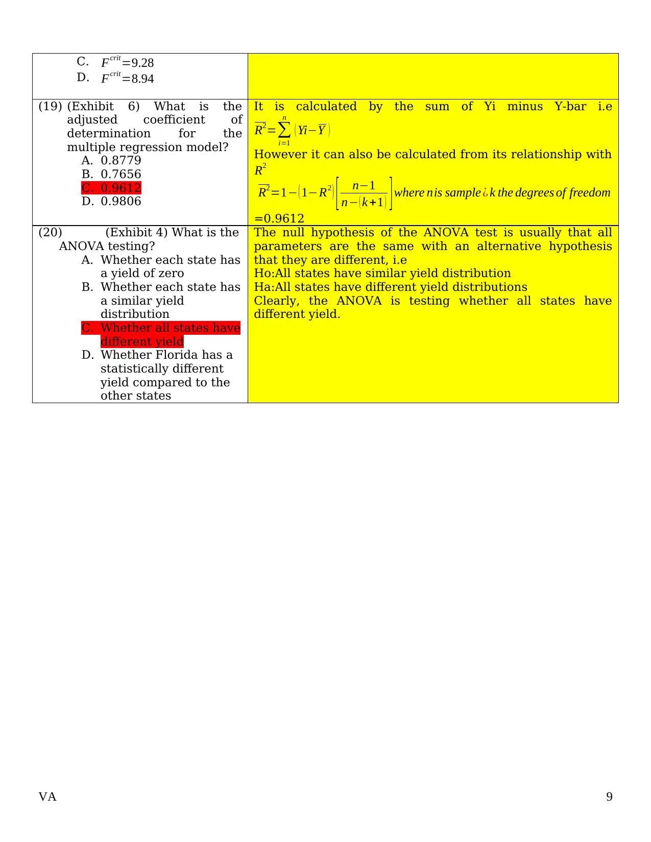
(19) (Exhibit 6) What is the
adjusted coefficient of
determination for the
multiple regression model?
A. 0.8779
B. 0.7656
C. 0.9612
D. 0.9806
It is calculated by the sum of Yi minus Y-bar i.e
R2=∑
i=1
n
( Yi−Y )
However it can also be calculated from its relationship with
R2
R2=1− ( 1−R2 ) [ n−1
n− ( k +1 ) ] where nis sample ¿ k the degrees of freedom
=0.9612
(20) (Exhibit 4) What is the
ANOVA testing?
A. Whether each state has
a yield of zero
B. Whether each state has
a similar yield
distribution
C. Whether all states have
different yield
D. Whether Florida has a
statistically different
yield compared to the
other states
The null hypothesis of the ANOVA test is usually that all
parameters are the same with an alternative hypothesis
that they are different, i.e
Ho:All states have similar yield distribution
Ha:All states have different yield distributions
Clearly, the ANOVA is testing whether all states have
different yield.
VA 9
D. Fcrit=8.94
(19) (Exhibit 6) What is the
adjusted coefficient of
determination for the
multiple regression model?
A. 0.8779
B. 0.7656
C. 0.9612
D. 0.9806
It is calculated by the sum of Yi minus Y-bar i.e
R2=∑
i=1
n
( Yi−Y )
However it can also be calculated from its relationship with
R2
R2=1− ( 1−R2 ) [ n−1
n− ( k +1 ) ] where nis sample ¿ k the degrees of freedom
=0.9612
(20) (Exhibit 4) What is the
ANOVA testing?
A. Whether each state has
a yield of zero
B. Whether each state has
a similar yield
distribution
C. Whether all states have
different yield
D. Whether Florida has a
statistically different
yield compared to the
other states
The null hypothesis of the ANOVA test is usually that all
parameters are the same with an alternative hypothesis
that they are different, i.e
Ho:All states have similar yield distribution
Ha:All states have different yield distributions
Clearly, the ANOVA is testing whether all states have
different yield.
VA 9
⊘ This is a preview!⊘
Do you want full access?
Subscribe today to unlock all pages.
Trusted by 1+ million students worldwide
1 out of 9
Your All-in-One AI-Powered Toolkit for Academic Success.
+13062052269
info@desklib.com
Available 24*7 on WhatsApp / Email
![[object Object]](/_next/static/media/star-bottom.7253800d.svg)
Unlock your academic potential
Copyright © 2020–2026 A2Z Services. All Rights Reserved. Developed and managed by ZUCOL.