Statistics for Management: Analysis of UK Earnings (2009-2016) Report
VerifiedAdded on 2021/02/19
|20
|3871
|47
Report
AI Summary
This Statistics for Management report analyzes earnings data, focusing on gender pay gaps in both public and private sectors. The report utilizes hypothesis testing to compare earnings, examining annual growth rates from 2009 to 2016. It includes calculations of mean, median, and standard deviation for hourly pay rates across different UK regions, along with quartile analysis and the creation of an ogive chart. The report also explores the concept of the Z-score, normal distribution, and economic order quantity. Furthermore, it presents charts and tables illustrating the relationship between the number of bedrooms and house prices in various streets, culminating in conclusions drawn from the statistical analysis.

STATISTICS FOR
MANAGEMENT
MANAGEMENT
Paraphrase This Document
Need a fresh take? Get an instant paraphrase of this document with our AI Paraphraser
TABLE OF CONTENTS
INTRODUCTION...........................................................................................................................3
MAIN BODY..................................................................................................................................3
TASK 1............................................................................................................................................3
A. Difference between earnings of men and women in public sector by testing of hypothesis. .3
B. Difference in the earnings of men and women in private sector through testing of
hypothesis....................................................................................................................................4
C. Earnings- Time Chart from 2009 to 2016...............................................................................5
D. Annual growth rate in earnings...............................................................................................7
TASK 2............................................................................................................................................8
Analysis and evaluation of hourly pay rates in different regions of UK.....................................8
TASK 3..........................................................................................................................................11
Section A...................................................................................................................................11
Section B....................................................................................................................................13
TASK 4..........................................................................................................................................13
Charts and Tables......................................................................................................................13
Relationship between the number of bedrooms and the price of houses in all the three streets16
CONCLUSION..............................................................................................................................17
REFERENCES................................................................................................................................1
Table 1: Public Sector Earnings of Men and Women................................................................4
Table 2: Earning in Private Sector...............................................................................................5
Table 3: Earnings in Public Sector...............................................................................................6
Table 4: Earnings in Private Sector.............................................................................................7
Table 5: Annual Growth Rate in Public Sector..........................................................................8
Table 6: Annual Growth Rate in Private Sector.........................................................................9
Table 7: Median Calculation of Hourly Earnings......................................................................9
Table 8: Calculation of Quartile Range.....................................................................................10
Table 9: Calculation of Arithmetic Mean..................................................................................11
Table 10: Calculation of Standard Deviation............................................................................11
Table 11: Comparison between Manchester and London.......................................................12
Table 12: Statistical Tables for Normal Distribution...............................................................13
Table 13: Economic Order Quantity.........................................................................................14
Table 14: Green Street Bedrooms..............................................................................................14
Table 15: Church Lane...............................................................................................................15
Table 16: Eton Avenue................................................................................................................16
Table 17: Percentage Change in Cost........................................................................................17
Figure 1: Normal Distribution Curve........................................................................................13
Figure 2: Cost of 2 and 3 Bedroom Houses in different Streets..............................................18
⊘ This is a preview!⊘
Do you want full access?
Subscribe today to unlock all pages.
Trusted by 1+ million students worldwide
INTRODUCTION
Statistics for management can be defined as those statistical tools and measures that
have been used in order to manage the business in a better manner and assists in formulating
better decisions. In this report, the comparison using different statistical tools will be made
between the earnings of men and women in both public as well as private sector businesses.
Further in this report, measures of central tendencies will be applied on the earnings of staff
workers in order to formulate correct interpretations. This is followed by the concept of Z score
and normal distribution curve and economic order quantity has also been discussed. Lastly, in
this report, various pie charts depicting the number of bedrooms will be presented followed by a
graph showing relationship between the number of bedrooms and the cost of these houses in
different streets.
MAIN BODY
TASK 1
A. Difference between earnings of men and women in public sector by testing of hypothesis
As per the question, the hypothesis that earnings of men and women do not exhibit any
significant difference needs to be tested (De Beer, Rothmann and Pienaar, 2016). Therefore,
Null Hypothesis (H0): The earnings of men and women working in public sector do not possess
any significant difference between them.
Alternate Hypothesis (H1): The earnings of men and women employed in public sector have
significant difference between them.
Table 1: Public Sector Earnings of Men and Women
t-Test of Two-
Sample
Assumption: Equal
Variance
Men's Earning in Public Sector Women's Earning in public sector
Mean 32276.625 26933.25
Variance 1449962.268 975692.5
Number of Years 8 8
Pooled Variance 1212827.384
Paraphrase This Document
Need a fresh take? Get an instant paraphrase of this document with our AI Paraphraser
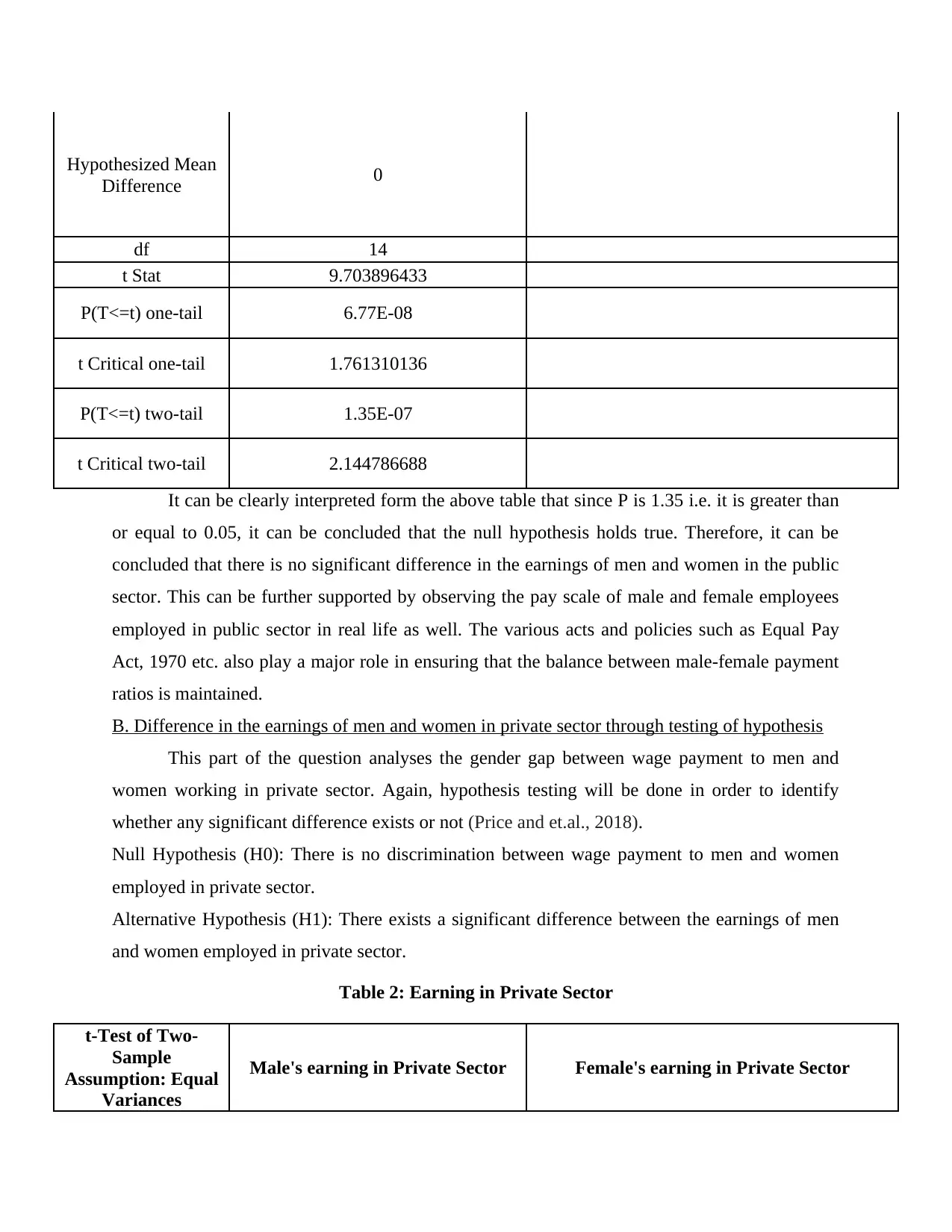
Hypothesized Mean
Difference 0
df 14
t Stat 9.703896433
P(T<=t) one-tail 6.77E-08
t Critical one-tail 1.761310136
P(T<=t) two-tail 1.35E-07
t Critical two-tail 2.144786688
It can be clearly interpreted form the above table that since P is 1.35 i.e. it is greater than
or equal to 0.05, it can be concluded that the null hypothesis holds true. Therefore, it can be
concluded that there is no significant difference in the earnings of men and women in the public
sector. This can be further supported by observing the pay scale of male and female employees
employed in public sector in real life as well. The various acts and policies such as Equal Pay
Act, 1970 etc. also play a major role in ensuring that the balance between male-female payment
ratios is maintained.
B. Difference in the earnings of men and women in private sector through testing of hypothesis
This part of the question analyses the gender gap between wage payment to men and
women working in private sector. Again, hypothesis testing will be done in order to identify
whether any significant difference exists or not (Price and et.al., 2018).
Null Hypothesis (H0): There is no discrimination between wage payment to men and women
employed in private sector.
Alternative Hypothesis (H1): There exists a significant difference between the earnings of men
and women employed in private sector.
Table 2: Earning in Private Sector
t-Test of Two-
Sample
Assumption: Equal
Variances
Male's earning in Private Sector Female's earning in Private Sector
Mean 28096.625 20541.25
Variance 795287.6964 988729.9286
Number of Years 8 8
Pooled Variance 892008.8125
Hypothesized Mean
Difference 0
df 14
t Stat 15.99931717
P(T<=t) one-tail 1.08E-10
t Critical one-tail 1.761310136
P(T<=t) two-tail 2.16E-10
t Critical two-tail 2.144786688
Again, it can be logically interpreted from the table prepared above that since the P is
2.16, which is again greater that 0.05, it can be significantly concluded that the null hypothesis
i.e. there is not any significant difference in the earnings of men and women working in the
private sector (Weakliem, 2016). Since the wage payment of employees has become highly
regulated and further, there is establishment of trade unions which are very active in supporting
and solving the grievances of the employees, private companies also ensure that they promote
the equal payment which improves their corporate image and assists them in refraining from
getting involved in any legal troubles ((Mankar, Shah and Lease, 2017)).
C. Earnings- Time Chart from 2009 to 2016
In this question, a graphical representation of the growth in earning of the male and
female employees from year 2019-16 has been presented for both public and private sector.
Table 3: Earnings in Public Sector
Year Male's Earnings Female's Earnings
2009 30638 25224
2010 31264 26113
2011 31380 26470
2012 31816 26663
2013 32541 27338
2014 32878 27705
2015 33685 27900
2016 34011 28053
⊘ This is a preview!⊘
Do you want full access?
Subscribe today to unlock all pages.
Trusted by 1+ million students worldwide
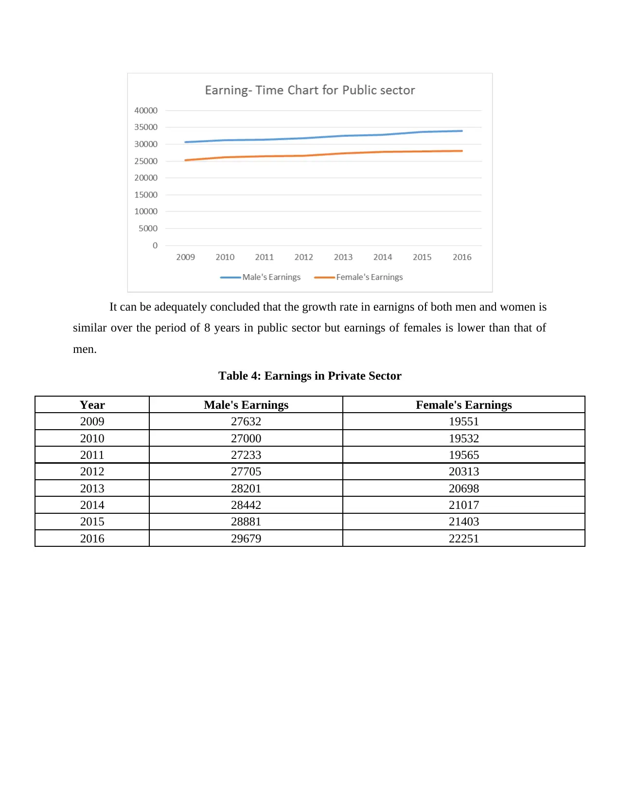
It can be adequately concluded that the growth rate in earnigns of both men and women is
similar over the period of 8 years in public sector but earnings of females is lower than that of
men.
Table 4: Earnings in Private Sector
Year Male's Earnings Female's Earnings
2009 27632 19551
2010 27000 19532
2011 27233 19565
2012 27705 20313
2013 28201 20698
2014 28442 21017
2015 28881 21403
2016 29679 22251
Paraphrase This Document
Need a fresh take? Get an instant paraphrase of this document with our AI Paraphraser
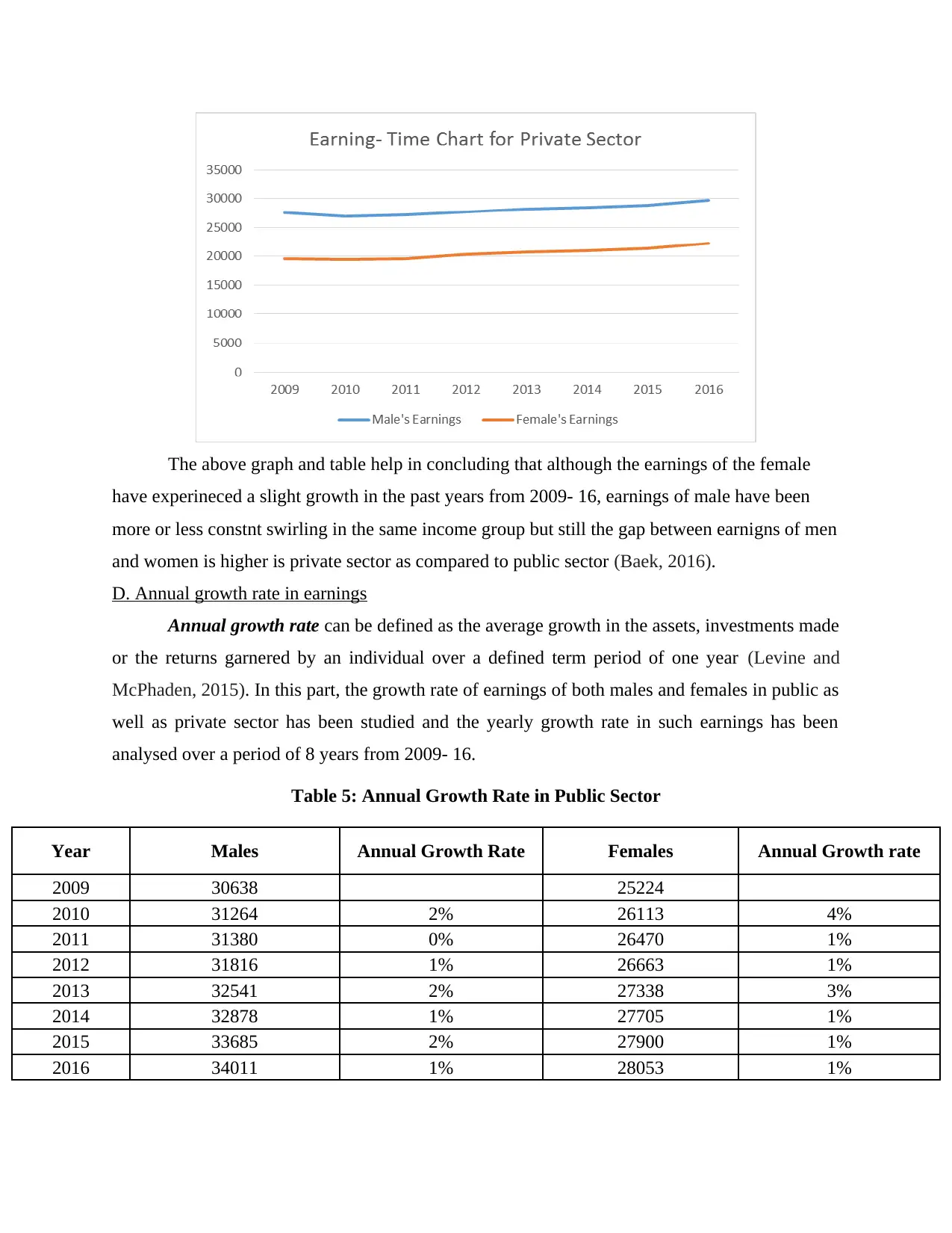
The above graph and table help in concluding that although the earnings of the female
have experineced a slight growth in the past years from 2009- 16, earnings of male have been
more or less constnt swirling in the same income group but still the gap between earnigns of men
and women is higher is private sector as compared to public sector (Baek, 2016).
D. Annual growth rate in earnings
Annual growth rate can be defined as the average growth in the assets, investments made
or the returns garnered by an individual over a defined term period of one year (Levine and
McPhaden, 2015). In this part, the growth rate of earnings of both males and females in public as
well as private sector has been studied and the yearly growth rate in such earnings has been
analysed over a period of 8 years from 2009- 16.
Table 5: Annual Growth Rate in Public Sector
Year Males Annual Growth Rate Females Annual Growth rate
2009 30638 25224
2010 31264 2% 26113 4%
2011 31380 0% 26470 1%
2012 31816 1% 26663 1%
2013 32541 2% 27338 3%
2014 32878 1% 27705 1%
2015 33685 2% 27900 1%
2016 34011 1% 28053 1%
It can be interpreted that while the growth rate men experiences less fluctuation, it is not
similar in the case of female who experience a higher fluctuation. However, the growth rate is
consistent over the time duration of 8 years in the time frame of 2009 to 2016.
Table 6: Annual Growth Rate in Private Sector
Year Males Annual Growth Rate Females Annual Growth Rate
2009 27632 19551
2010 27000 -2% 19532 0%
2011 27233 1% 19565 0%
2012 27705 2% 20313 4%
2013 28201 2% 20698 2%
2014 28442 1% 21017 2%
2015 28881 2% 21403 2%
2016 29679 3% 22251 4%
Further from the above table it can be again interpreted that although there is fluctuation
in both Men’s as well as Women’s Growth Rate in some particular years, overall the growth rate
has remained constant. However, growth rate of women is much lower as compared to women
and the difference is more pronounced especially in private sector.
TASK 2
Analysis and evaluation of hourly pay rates in different regions of UK
In this question, the mean, median and standard deviation of the earnings per hour basis
are taken and quartiles are depicted through an ogive chart.
Median and Quartile estimation of Hourly earnings:
Median can be defined as that value which lies exactly in the middle of a range or series
of data which have been arranged in ascending or descending order (Daskin and Maass, 2015).
When the number of observations is odd, the middle number is selected is median and when
observations are even, median is calculated by taking the average of two middle values.
Table 7: Median Calculation of Hourly Earnings
Hourly earning Leisure Centre Staff (f) Cumulative frequency (cf)
0 – 10 4 4
10 – 20 23 27
20 – 30 13 40
⊘ This is a preview!⊘
Do you want full access?
Subscribe today to unlock all pages.
Trusted by 1+ million students worldwide
30 – 40 7 47
40 – 50 3 50
Median can be calculated through division of the last cumulative frequency by 2 i.e. 50/2
which is 25. Therefore, the median of leisure centre staff is 25.
Quartile is another measure and under this, data is divided into four intervals and then
these sets are compared to draw relevant conclusions. Interquartile range is subtraction of
Quartile 1 form Quartile 3 i.e. Q3-Q1 (Luo and et.al., 2018).
Table 8: Calculation of Quartile Range
1 Quartile 4
3 Quartile 13
Interquartile Range 9
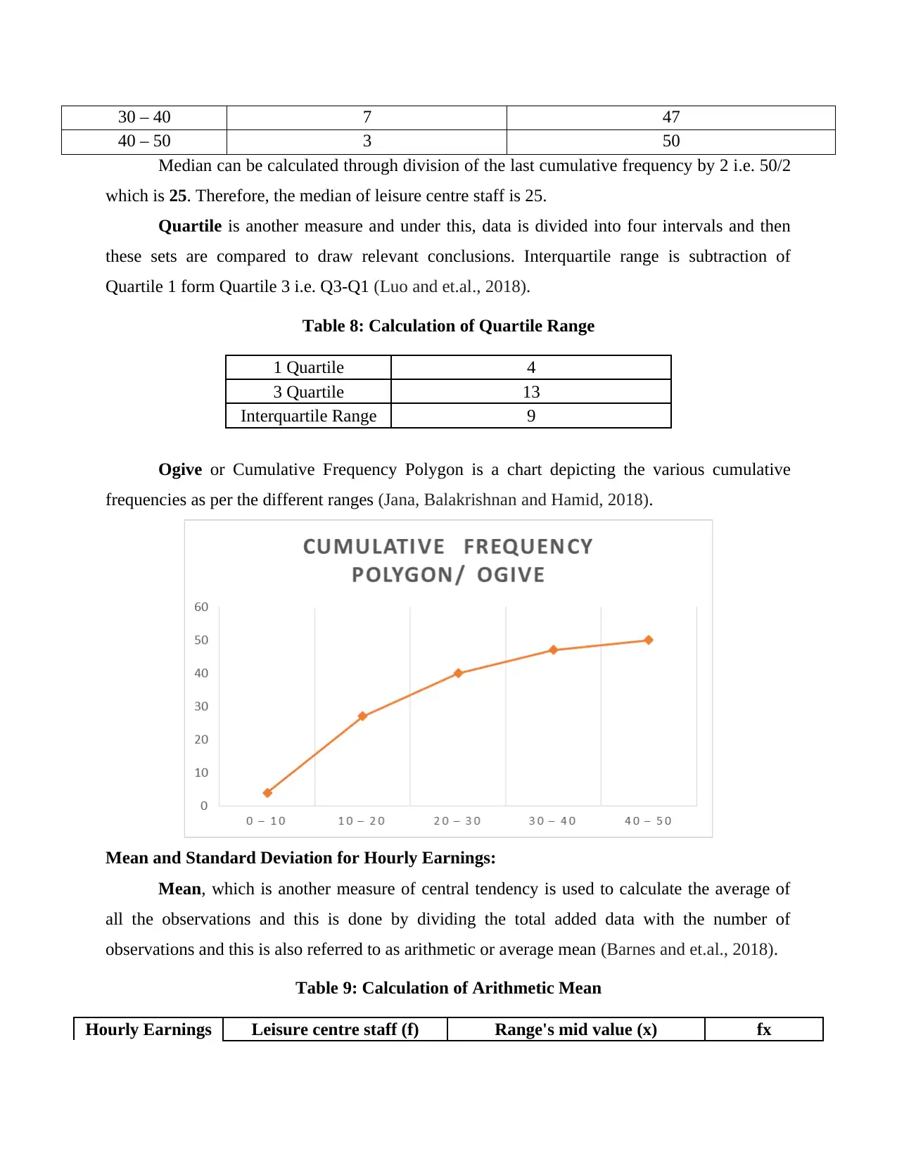
Ogive or Cumulative Frequency Polygon is a chart depicting the various cumulative
frequencies as per the different ranges (Jana, Balakrishnan and Hamid, 2018).
Mean and Standard Deviation for Hourly Earnings:
Mean, which is another measure of central tendency is used to calculate the average of
all the observations and this is done by dividing the total added data with the number of
observations and this is also referred to as arithmetic or average mean (Barnes and et.al., 2018).
Table 9: Calculation of Arithmetic Mean
Hourly Earnings Leisure centre staff (f) Range's mid value (x) fx
40 – 50 3 50
Median can be calculated through division of the last cumulative frequency by 2 i.e. 50/2
which is 25. Therefore, the median of leisure centre staff is 25.
Quartile is another measure and under this, data is divided into four intervals and then
these sets are compared to draw relevant conclusions. Interquartile range is subtraction of
Quartile 1 form Quartile 3 i.e. Q3-Q1 (Luo and et.al., 2018).
Table 8: Calculation of Quartile Range
1 Quartile 4
3 Quartile 13
Interquartile Range 9
Ogive or Cumulative Frequency Polygon is a chart depicting the various cumulative
frequencies as per the different ranges (Jana, Balakrishnan and Hamid, 2018).
Mean and Standard Deviation for Hourly Earnings:
Mean, which is another measure of central tendency is used to calculate the average of
all the observations and this is done by dividing the total added data with the number of
observations and this is also referred to as arithmetic or average mean (Barnes and et.al., 2018).
Table 9: Calculation of Arithmetic Mean
Hourly Earnings Leisure centre staff (f) Range's mid value (x) fx
Paraphrase This Document
Need a fresh take? Get an instant paraphrase of this document with our AI Paraphraser
0 – 10 4 5 20
10 – 20 23 15 345
20 – 30 13 25 325
30 – 40 7 35 245
40 – 50 3 45 135
Total 50 1070
Here, arithmetic mean can be calculated as division of total of fx column from f i.e.
Σfx/Σf. Therefore, the mean is 1070/ 50= 21.4.
It can be concluded from the above data that mean (x̄) which is 21.4 i.e. the hourly
earnings of the leisure staff in UK is lying within the range of 20-30. It must be noted that the
value of mean is always fixed i.e. it will not change with the changes in staff frequency.
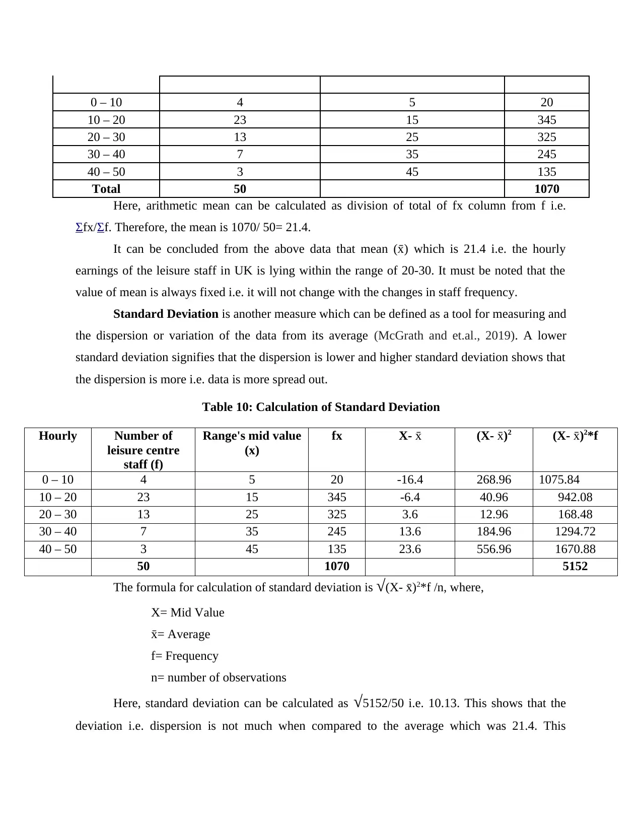
Standard Deviation is another measure which can be defined as a tool for measuring and
the dispersion or variation of the data from its average (McGrath and et.al., 2019). A lower
standard deviation signifies that the dispersion is lower and higher standard deviation shows that
the dispersion is more i.e. data is more spread out.
Table 10: Calculation of Standard Deviation
Hourly Number of
leisure centre
staff (f)
Range's mid value
(x)
fx X- x̄ (X- x̄)2 (X- x̄)2*f
0 – 10 4 5 20 -16.4 268.96 1075.84
10 – 20 23 15 345 -6.4 40.96 942.08
20 – 30 13 25 325 3.6 12.96 168.48
30 – 40 7 35 245 13.6 184.96 1294.72
40 – 50 3 45 135 23.6 556.96 1670.88
50 1070 5152
The formula for calculation of standard deviation is √(X- x̄)2*f /n, where,
X= Mid Value
x̄= Average
f= Frequency
n= number of observations
Here, standard deviation can be calculated as √5152/50 i.e. 10.13. This shows that the
deviation i.e. dispersion is not much when compared to the average which was 21.4. This
10 – 20 23 15 345
20 – 30 13 25 325
30 – 40 7 35 245
40 – 50 3 45 135
Total 50 1070
Here, arithmetic mean can be calculated as division of total of fx column from f i.e.
Σfx/Σf. Therefore, the mean is 1070/ 50= 21.4.
It can be concluded from the above data that mean (x̄) which is 21.4 i.e. the hourly
earnings of the leisure staff in UK is lying within the range of 20-30. It must be noted that the
value of mean is always fixed i.e. it will not change with the changes in staff frequency.
Standard Deviation is another measure which can be defined as a tool for measuring and
the dispersion or variation of the data from its average (McGrath and et.al., 2019). A lower
standard deviation signifies that the dispersion is lower and higher standard deviation shows that
the dispersion is more i.e. data is more spread out.
Table 10: Calculation of Standard Deviation
Hourly Number of
leisure centre
staff (f)
Range's mid value
(x)
fx X- x̄ (X- x̄)2 (X- x̄)2*f
0 – 10 4 5 20 -16.4 268.96 1075.84
10 – 20 23 15 345 -6.4 40.96 942.08
20 – 30 13 25 325 3.6 12.96 168.48
30 – 40 7 35 245 13.6 184.96 1294.72
40 – 50 3 45 135 23.6 556.96 1670.88
50 1070 5152
The formula for calculation of standard deviation is √(X- x̄)2*f /n, where,
X= Mid Value
x̄= Average
f= Frequency
n= number of observations
Here, standard deviation can be calculated as √5152/50 i.e. 10.13. This shows that the
deviation i.e. dispersion is not much when compared to the average which was 21.4. This
signifies that the deviation between earnings of the leisure staff is low when compared to the
average earnings.
Earnings of leisure staff in Manchester:
In this question, a comp0arison has been made on the basis of measures of central
tendency pertaining to the data related to the leisure staff in Manchester and London.
Table 11: Comparison between Manchester and London
Particulars London Manchester
Median 14.13 14
Interquartile Range 9 7.5
Mean 21.4 16.5
Standard deviation 10.13 7
From the above chart showing comparison of the values, it can be clearly ascertained that
the median which depicts the middle value of the earnings is almost similar depicted as 14.13 in
London and 14 in Manchester. The mean i.e. the average earnings of Leisure workers in London
is higher at 9 when compared to that of Manchester which is 7.5. This can be due to London
being a more developed and tourist attracting city. The standard deviation depicting the
dispersion or variance of London which is 10.13 is higher than that of Manchester which is 7 and
this increase in fluctuation can be due to variation in earnings in the tourist season v/s off season
(Ross, 2017).
TASK 3
Section A
Normal Distribution Curve is a continuous probability distribution curve which is often
used to represent distribution of random variables with real values (Jana, Balakrishnan and
Hamid, 2018).
⊘ This is a preview!⊘
Do you want full access?
Subscribe today to unlock all pages.
Trusted by 1+ million students worldwide
1 out of 20
Related Documents


Your All-in-One AI-Powered Toolkit for Academic Success.
+13062052269
info@desklib.com
Available 24*7 on WhatsApp / Email
![[object Object]](/_next/static/media/star-bottom.7253800d.svg)
Unlock your academic potential
Copyright © 2020–2026 A2Z Services. All Rights Reserved. Developed and managed by ZUCOL.