Comprehensive Report on Understanding and Managing Data Sets

This report provides a comprehensive analysis of understanding and managing data, covering various statistical tools and techniques. It includes calculations of mean, standard deviation, interquartile range, and coefficient of variation for a given dataset. The report discusses the differences between cross-sectional and time series data, highlighting their applications in understanding consumer characteristics. A project schedule with critical path analysis is presented, along with a correlation matrix analyzing factors affecting job separation. Regression analysis is performed, and the high-low method is used to analyze cost behavior. The report concludes with reflections on the learning experience and suggestions for future improvements. Access similar solved assignments on Desklib.

Understanding and Managing
Data

TABLE OF CONTENTS
PART 1............................................................................................................................................3
Task 1..........................................................................................................................................3
Task 2..........................................................................................................................................3
Task 3..........................................................................................................................................4
Task 4..........................................................................................................................................5
Task 5..........................................................................................................................................6
Task 6..........................................................................................................................................8
PART 2............................................................................................................................................8
1...................................................................................................................................................9
2...................................................................................................................................................9
3...................................................................................................................................................9
4...................................................................................................................................................9
5...................................................................................................................................................9
6...................................................................................................................................................9
REFERENCES..............................................................................................................................11

PART 1
Task 1
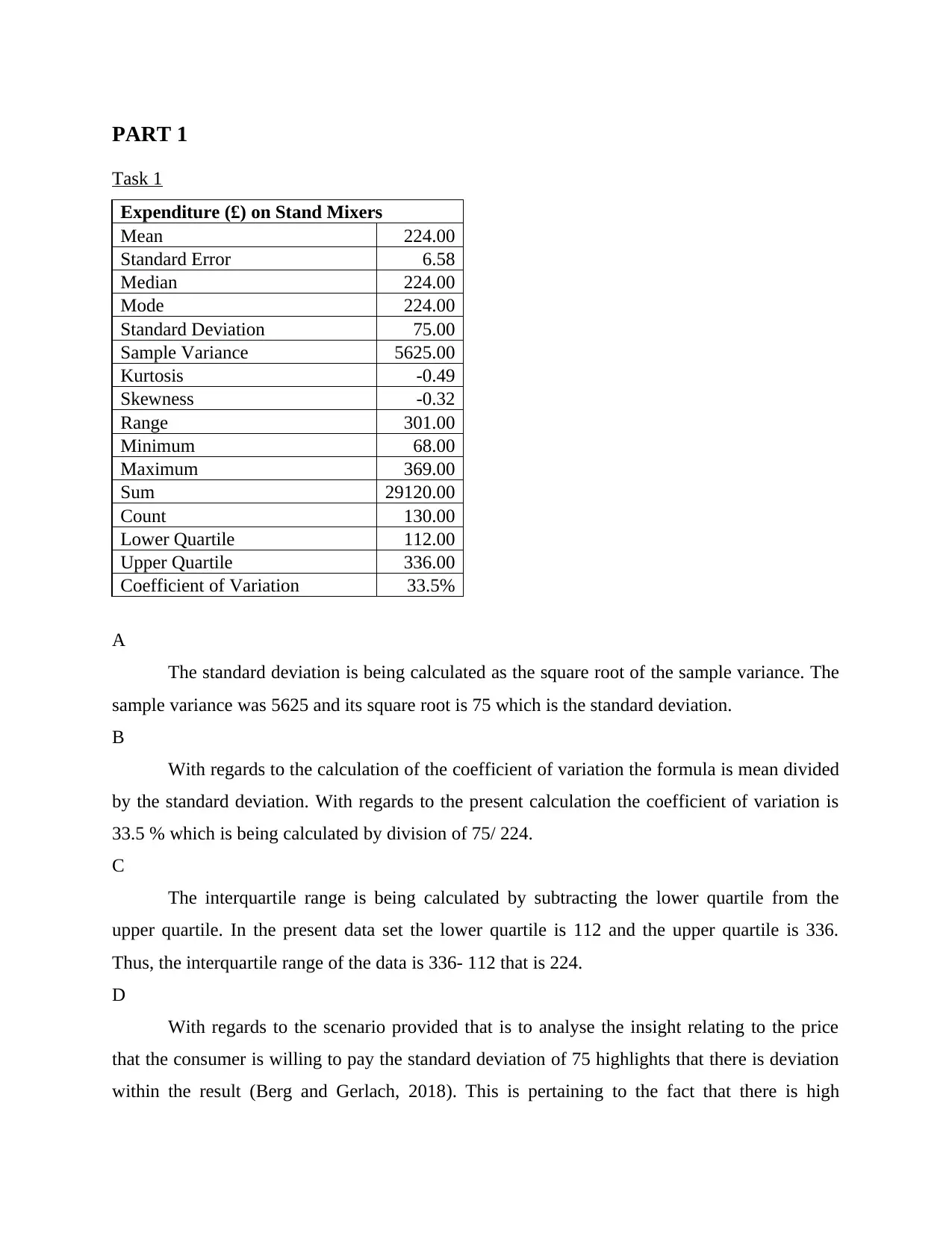
Expenditure (£) on Stand Mixers
Mean 224.00
Standard Error 6.58
Median 224.00
Mode 224.00
Standard Deviation 75.00
Sample Variance 5625.00
Kurtosis -0.49
Skewness -0.32
Range 301.00
Minimum 68.00
Maximum 369.00
Sum 29120.00
Count 130.00
Lower Quartile 112.00
Upper Quartile 336.00
Coefficient of Variation 33.5%
A
The standard deviation is being calculated as the square root of the sample variance. The
sample variance was 5625 and its square root is 75 which is the standard deviation.
B
With regards to the calculation of the coefficient of variation the formula is mean divided
by the standard deviation. With regards to the present calculation the coefficient of variation is
33.5 % which is being calculated by division of 75/ 224.
C
The interquartile range is being calculated by subtracting the lower quartile from the
upper quartile. In the present data set the lower quartile is 112 and the upper quartile is 336.
Thus, the interquartile range of the data is 336- 112 that is 224.
D
With regards to the scenario provided that is to analyse the insight relating to the price
that the consumer is willing to pay the standard deviation of 75 highlights that there is deviation
within the result (Berg and Gerlach, 2018). This is pertaining to the fact that there is high

deviation being present in the values of the data and the answer will also be deviating to a great
extent.
E
The interquartile range outlines that where the mid fifty of the data is being present in the
whole data set. In this present set the interquartile range is 224 and this means that the data lies in
between this data set.
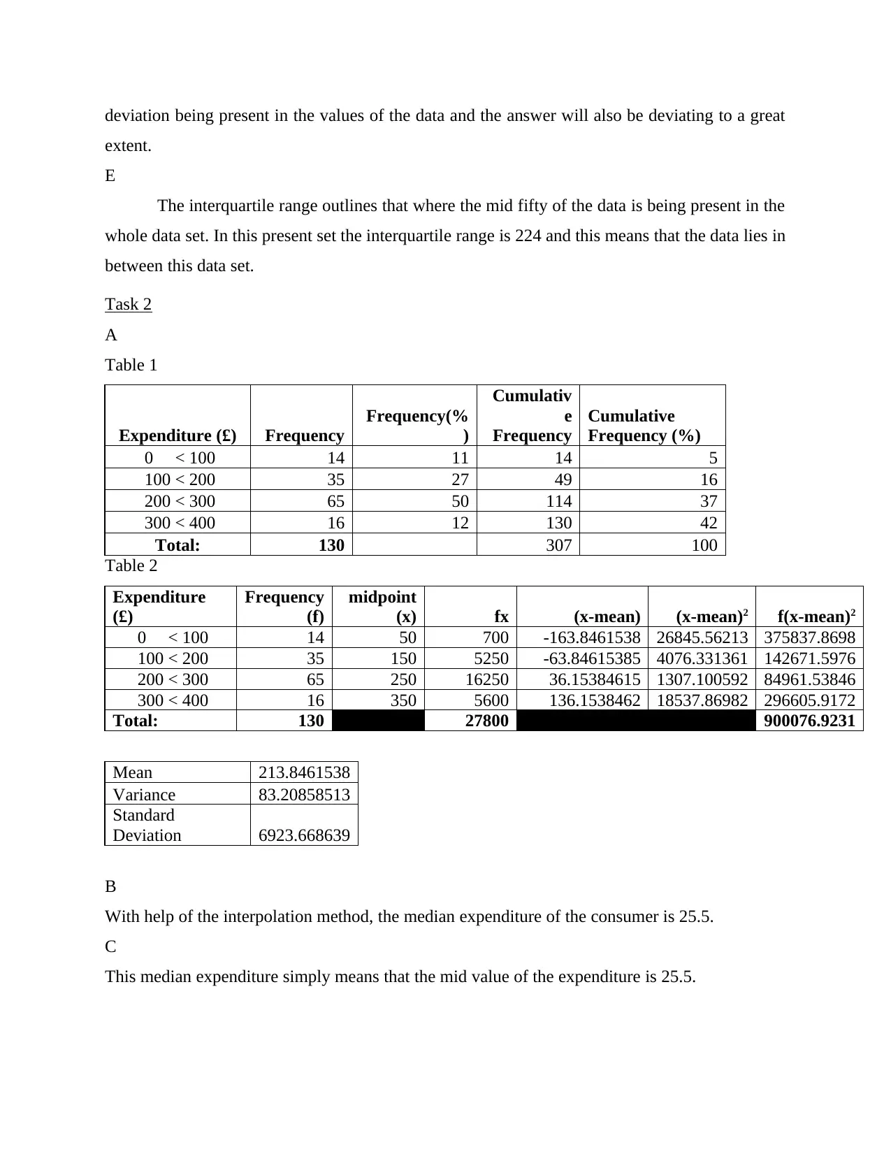
Task 2
A
Table 1
Expenditure (£) Frequency
Frequency(%
)
Cumulativ
e
Frequency
Cumulative
Frequency (%)
0 < 100 14 11 14 5
100 < 200 35 27 49 16
200 < 300 65 50 114 37
300 < 400 16 12 130 42
Total: 130 307 100
Table 2
Expenditure
(£)
Frequency
(f)
midpoint
(x) fx (x-mean) (x-mean)2 f(x-mean)2
0 < 100 14 50 700 -163.8461538 26845.56213 375837.8698
100 < 200 35 150 5250 -63.84615385 4076.331361 142671.5976
200 < 300 65 250 16250 36.15384615 1307.100592 84961.53846
300 < 400 16 350 5600 136.1538462 18537.86982 296605.9172
Total: 130 27800 900076.9231
Mean 213.8461538
Variance 83.20858513
Standard
Deviation 6923.668639
B
With help of the interpolation method, the median expenditure of the consumer is 25.5.
C
This median expenditure simply means that the mid value of the expenditure is 25.5.

Task 3
A
There is a difference being present within the cross- sectional data and the time series
data. The major difference being present between both of them is that the time series data is the
one which includes same variable over the particular period of time. On the other hand, the cross
sectional data is the one which use the different set of data but at a particular given point of time
only.
B
With regards to the present case provided for understanding the target consumer and the
insight of consumer characteristic the use of cross- sectional data will be used. This is because of
the reason that when the working of the company will be using this data then they will be
providing a better overview of the characteristic of the consumers (Raymond and et.al., 2020).
Along with this the time series data will also be helpful for the company to analyse the trend of
the consumer over the period of time. Thus, it can be stated that overall the combination of the
both the cross sectional and time series data will be used in order to collect the data relating to
the insight into the demographic profile and the lifestyle preference of the consumers.
Task 4
Task
Mode Task Name Duration Start Finish Predecessors
Auto
Scheduled A 6 wks Thu 7/21/22 Wed 8/31/22
Auto
Scheduled B 4 days Thu 7/21/22 Tue 7/26/22
Auto
Scheduled C 4 days Thu 9/1/22 Tue 9/6/22 1
Auto
Scheduled D 2 days Wed 7/27/22 Thu 7/28/22 2
Auto
Scheduled E 6 days Wed 9/7/22 Wed 9/14/22 3
Auto
Scheduled F 5 days Wed 9/7/22 Tue 9/13/22 3,4
Auto
Scheduled G 3 days Fri 7/29/22 Tue 8/2/22 4
Auto
Scheduled H 8 days Thu 7/21/22 Mon 8/1/22

Auto
Scheduled I 5 days Thu 9/15/22 Wed 9/21/22 5,6,7
Auto
Scheduled J 2 days Thu 9/22/22 Fri 9/23/22 8,9
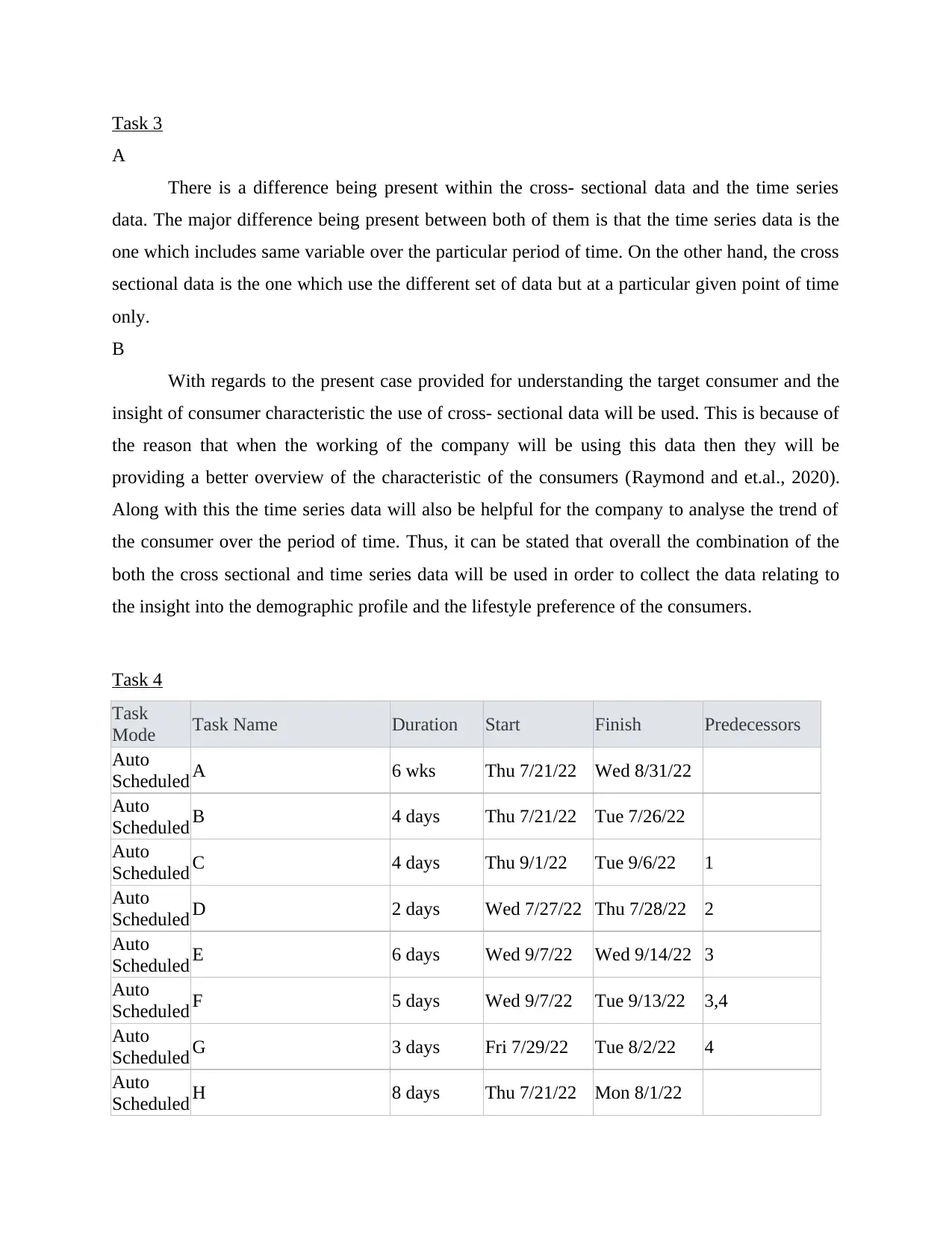
The critical path of the project involves the following activities
1 + 3 + 5 + 9 + 10
So the total week for critical path involves-
6 + 4 + 6 + 5 + 2
= 23 weeks
D
The major difference between the critical activities and the non critical activities this that
any change within the critical activity will be delaying the project to a great extent. On the other
hand any change within the non critical activity will not be causing any change over theme
working of the critical path or the activities of the business.
Task 5
A
Job
Separation*
(Probability)
Workers'
Age
Gross
Hourly Pay
(£)
Commuting
Time
(Minutes)
Average
Weekly
Hours of
Work
Job Separation*
(Probability) 1
Workers' Age
-
0.850933508 1
Gross Hourly Pay
(£)
-
0.780425444 0.526156257 1
Commuting Time
(Minutes) 0.862105058
-
0.782546734
-
0.682470154 1

Average Weekly
Hours of Work
-
0.180338317
-
0.029551426 0.377466662 0.017314834 1
B
The best predictor of the correlation matrix is the commuting time. This is particularly
because of the reason that the core relation between job separation and the commuting time as
86% which was highly correlated. This with this it can be implied that the best product for the
job separation is the commuting time.
C
D
With the help of correlation matrix it can be evaluated that mostly all the factors are
having negative correlation among themselves. Only the factors like job separation and
commuting time along with average weekly hours of work is having positive relation. Along
with this workers age and gross salary have positive correlation (Gremler and et.al., 2020). along
with average weekly hours is also having some positive cross hourly pay is positively core
related with the average weekly hours of work. Further the commuting time is correlated with
average weekly hours of. But most of the cases there is negative correlation like in case of
workers age and the jobs separation.
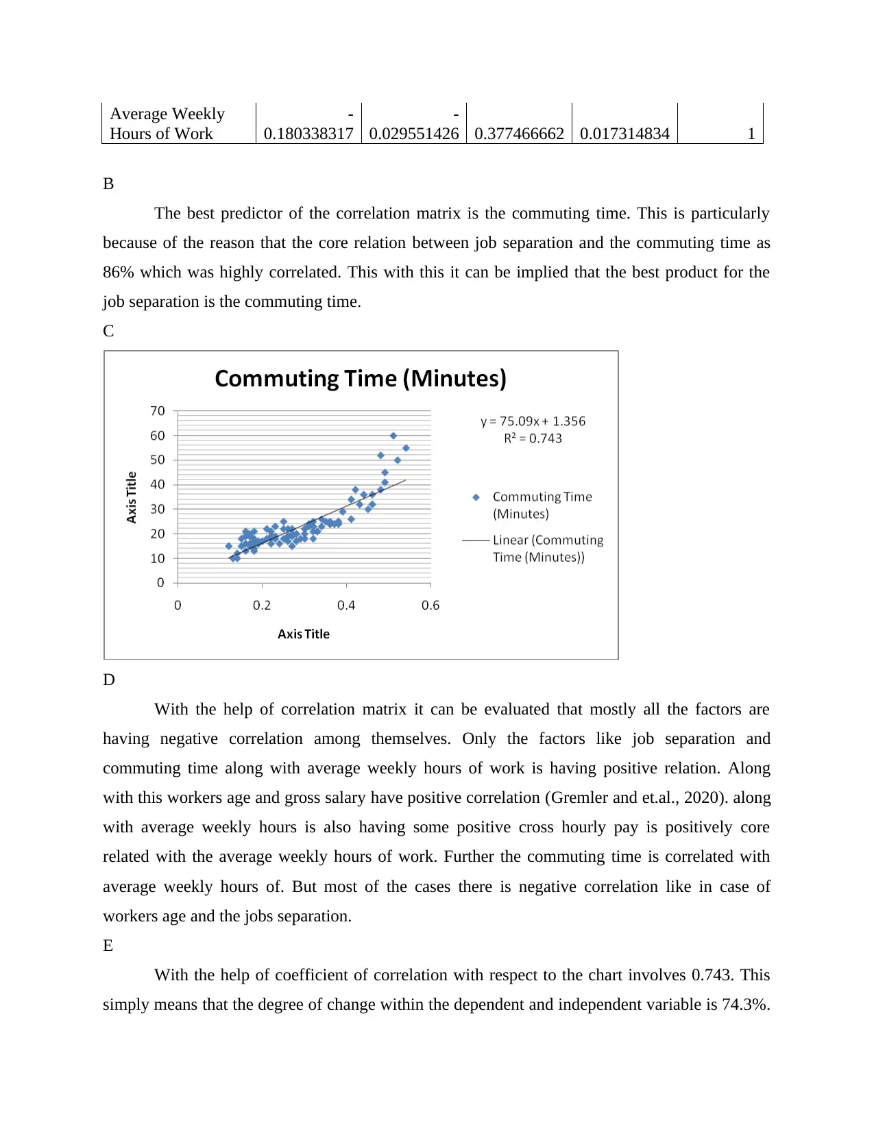
E
With the help of coefficient of correlation with respect to the chart involves 0.743. This
simply means that the degree of change within the dependent and independent variable is 74.3%.

Hence the simply means that when there will be any change in the Independence variable then it
will be causing a change of 74.3% into the dependent variable as well.
F
y = 75.09x + 1.356
G
The value of intercept within the regression equation is 75.09 X. The simply means that
the value which will be predicted will be placed in the category of X and will be multiplied by
75.09.
H
Along with this the gradient with context to the regression equation involves the value
1.356. Hence the simply means that this value will be added within the multiplication of 75.09
and the value of X is added up. this simply implies that when the gradient and intercept are being
added then the value of Y is being calculated.
Task 6
1
The thing which went well in the study was the fact that knowledge relating to the
different types of the statistical tools and techniques was enhanced. This simply implies that with
help of this assignment the knowledge relating to the various tools and techniques of statistics
was used and this improved the knowledge. along with this the researching skills was also
improved as the different statistical tools need to be researched in better and effective manner.
Hence, with this the researching skills has improved and this will be assisting in improving the
working efficiency in the future as well.
2
The most challenging aspect within the coursework was the selection of the appropriate
data and tool to analyse it. This is pertaining to the fact that the data is tough to find and also it is
hard to find the appropriate statistical tool for analysing the data (Kienecker, Sedlacek and
Turner, 2018). Hence, this was the most challenging task and resulted in increase in time for the
selection of appropriate tools. But with good researching skills I was able to analyse and evaluate
the appropriate data and tool to analyse it in proper and effective manner.
3

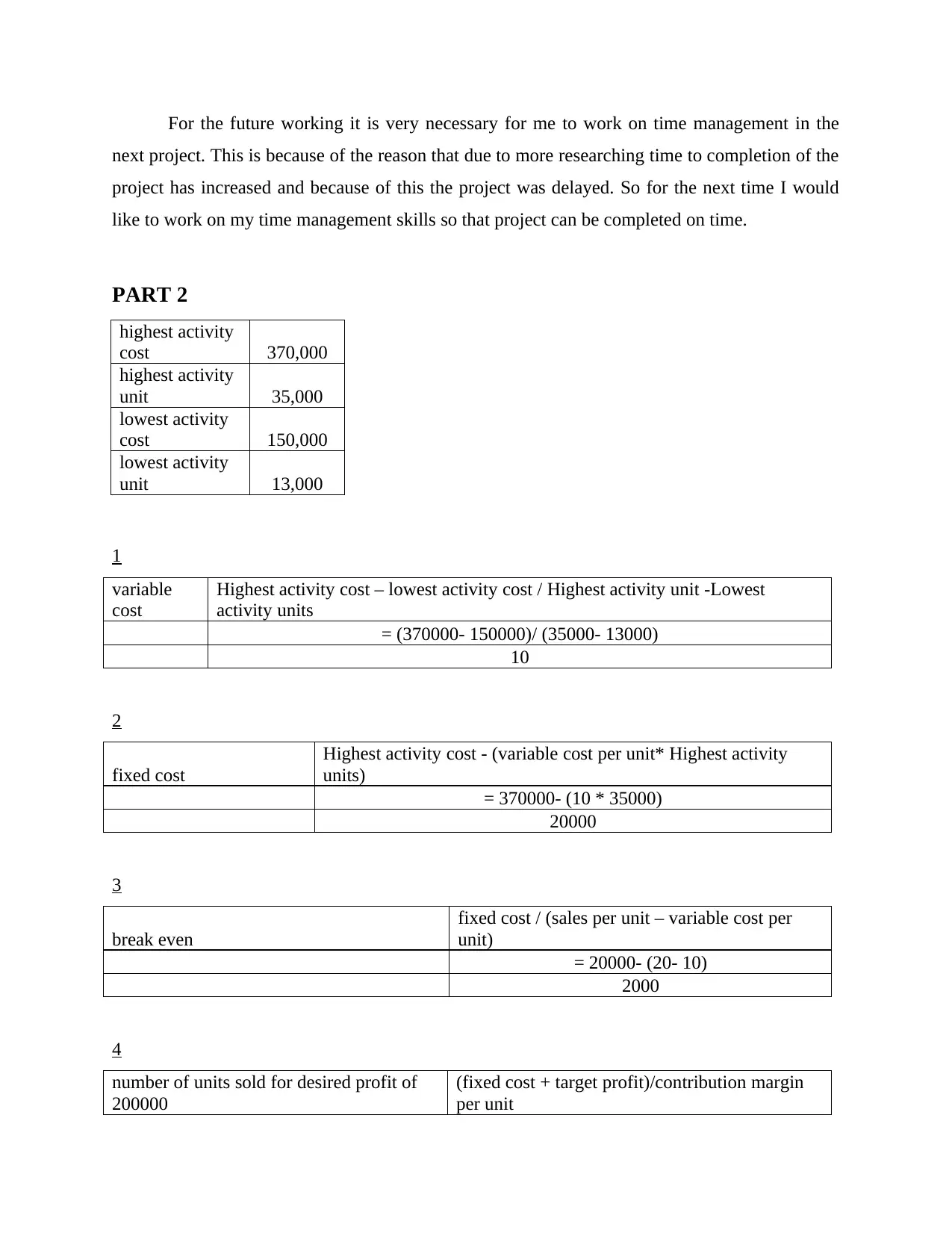
For the future working it is very necessary for me to work on time management in the
next project. This is because of the reason that due to more researching time to completion of the
project has increased and because of this the project was delayed. So for the next time I would
like to work on my time management skills so that project can be completed on time.
PART 2
highest activity
cost 370,000
highest activity
unit 35,000
lowest activity
cost 150,000
lowest activity
unit 13,000
1
variable
cost
Highest activity cost – lowest activity cost / Highest activity unit -Lowest
activity units
= (370000- 150000)/ (35000- 13000)
10
2
fixed cost
Highest activity cost - (variable cost per unit* Highest activity
units)
= 370000- (10 * 35000)
20000
3
break even
fixed cost / (sales per unit – variable cost per
unit)
= 20000- (20- 10)
2000
4
number of units sold for desired profit of
200000
(fixed cost + target profit)/contribution margin
per unit

= (20000 + 200000)/ 10
22000
5
Margin of safety actual sales- break even sales
= 24800 - 22000
2,800
6
A
High- low method is being used in the present situation because here the variable cost
and the fixed cost were not provided and only the level of activities and unit was provided.
Hence for this the use of high- low method is very beneficial for calculating the variable cost and
fixed cost.
B
The value of margin of safety outlines that how much the company can lose in its sales
before the company start losing the money. This simply means that higher the margin of safety
the lower is the risk of not breaking even or anchoring or lost (Pangrazio and Selwyn, 2019).
Hence the margin of safety is 2800 which implies that this much is the value up to which the
company will not be incurring the loss.
C
The major importance of break even analysis that it assist the company in evaluating an
identifying the level of production and which they will be in position of no profit no loss.

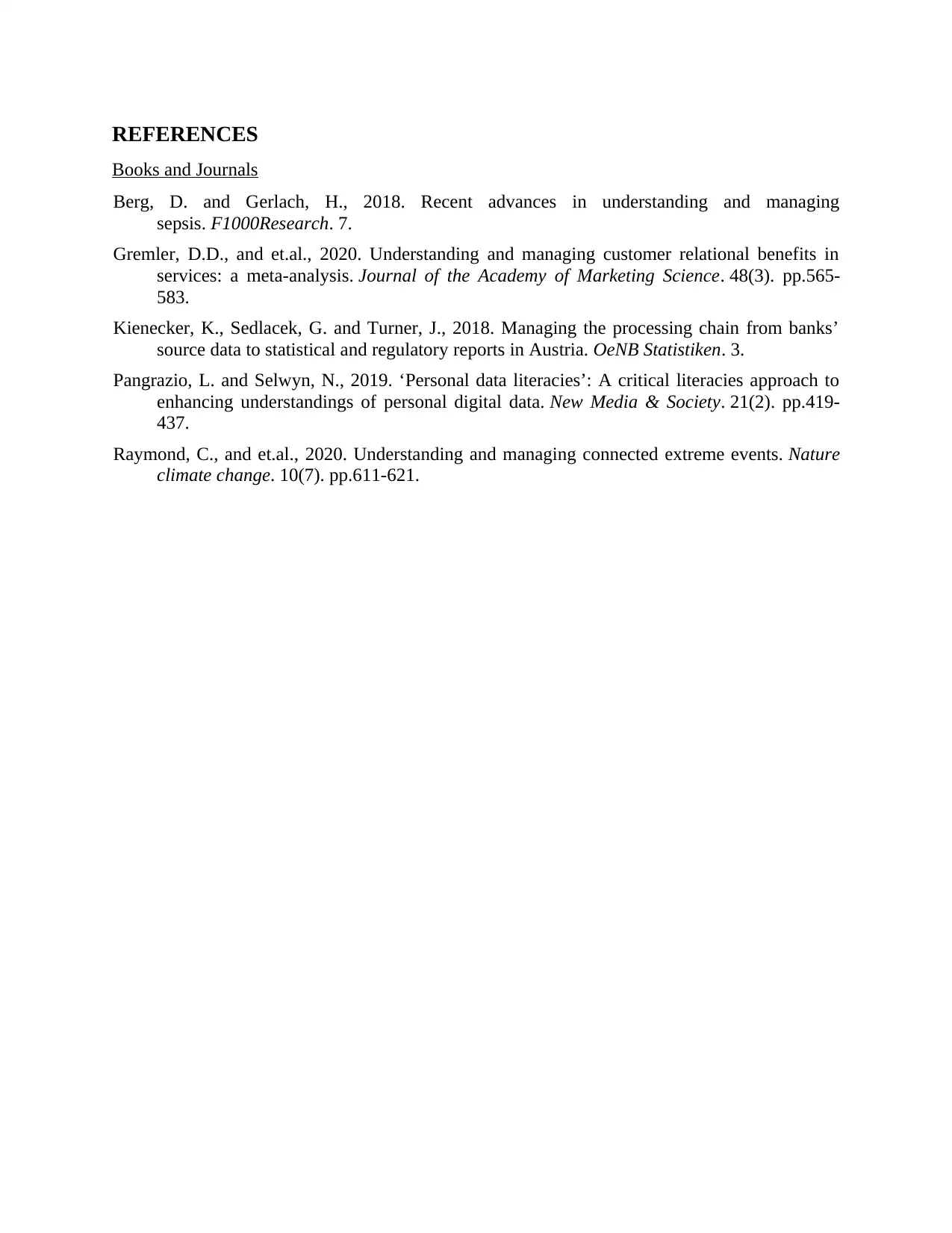
REFERENCES
Books and Journals
Berg, D. and Gerlach, H., 2018. Recent advances in understanding and managing
sepsis. F1000Research. 7.
Gremler, D.D., and et.al., 2020. Understanding and managing customer relational benefits in
services: a meta-analysis. Journal of the Academy of Marketing Science. 48(3). pp.565-
583.
Kienecker, K., Sedlacek, G. and Turner, J., 2018. Managing the processing chain from banks’
source data to statistical and regulatory reports in Austria. OeNB Statistiken. 3.
Pangrazio, L. and Selwyn, N., 2019. ‘Personal data literacies’: A critical literacies approach to
enhancing understandings of personal digital data. New Media & Society. 21(2). pp.419-
437.
Raymond, C., and et.al., 2020. Understanding and managing connected extreme events. Nature
climate change. 10(7). pp.611-621.