University Statistics: AMOS Analysis of Model Fit and Comparison

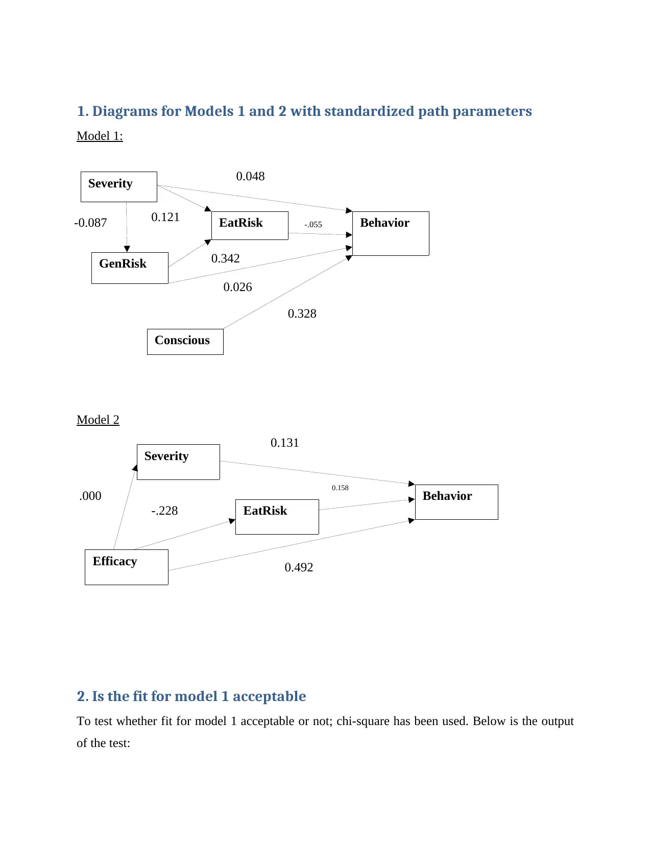
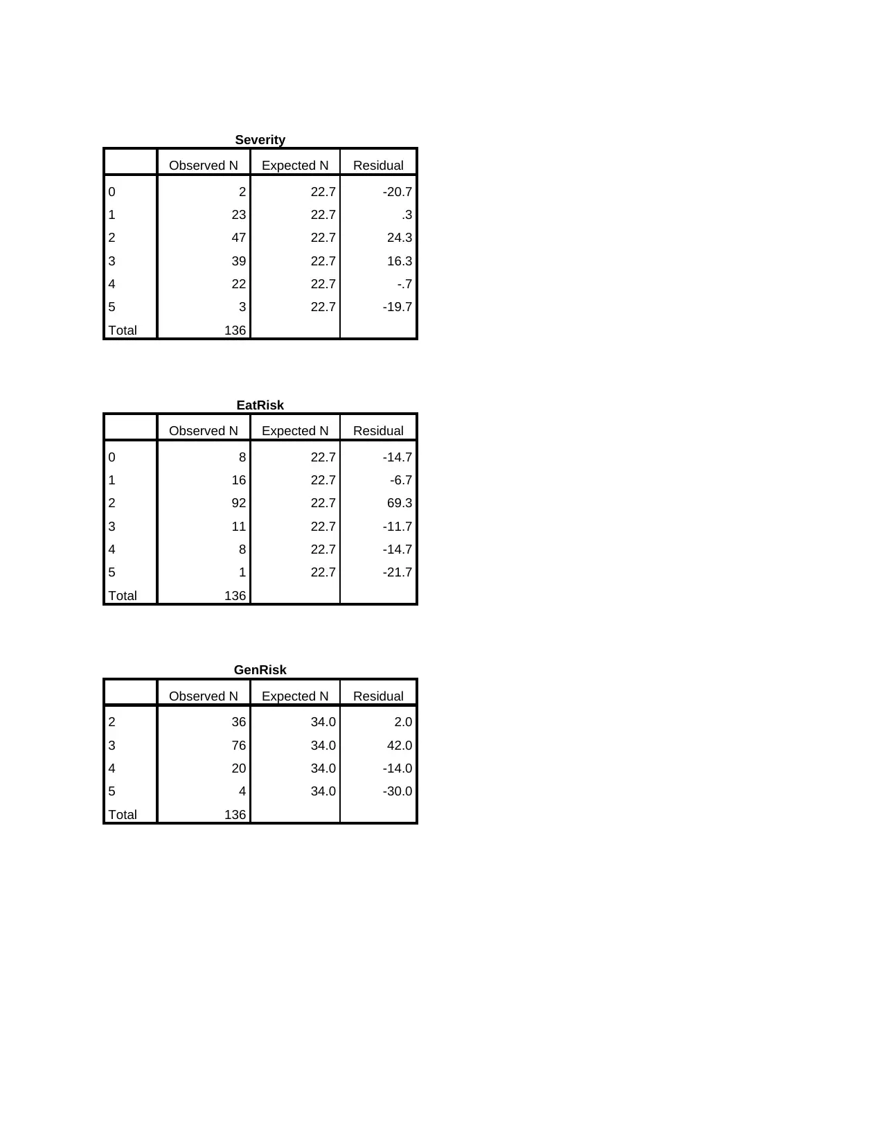
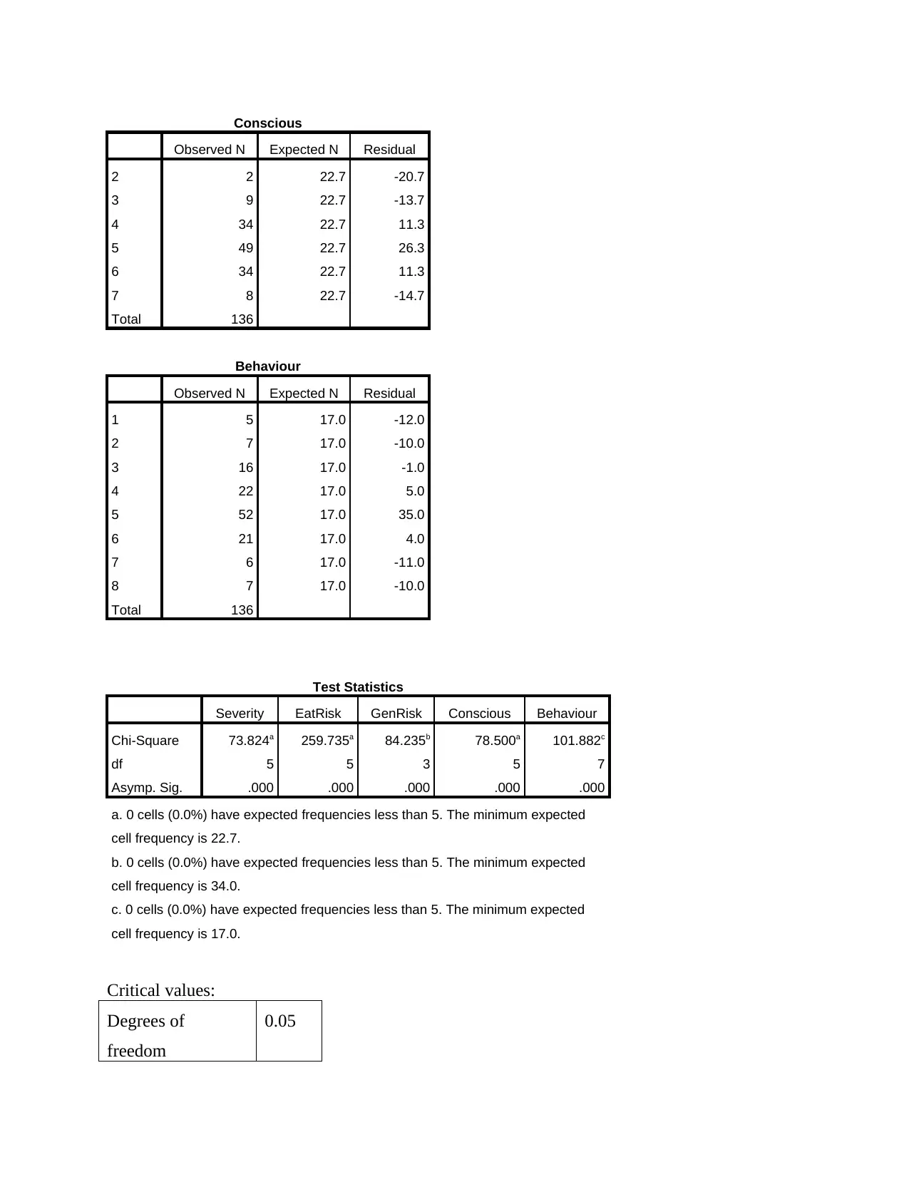
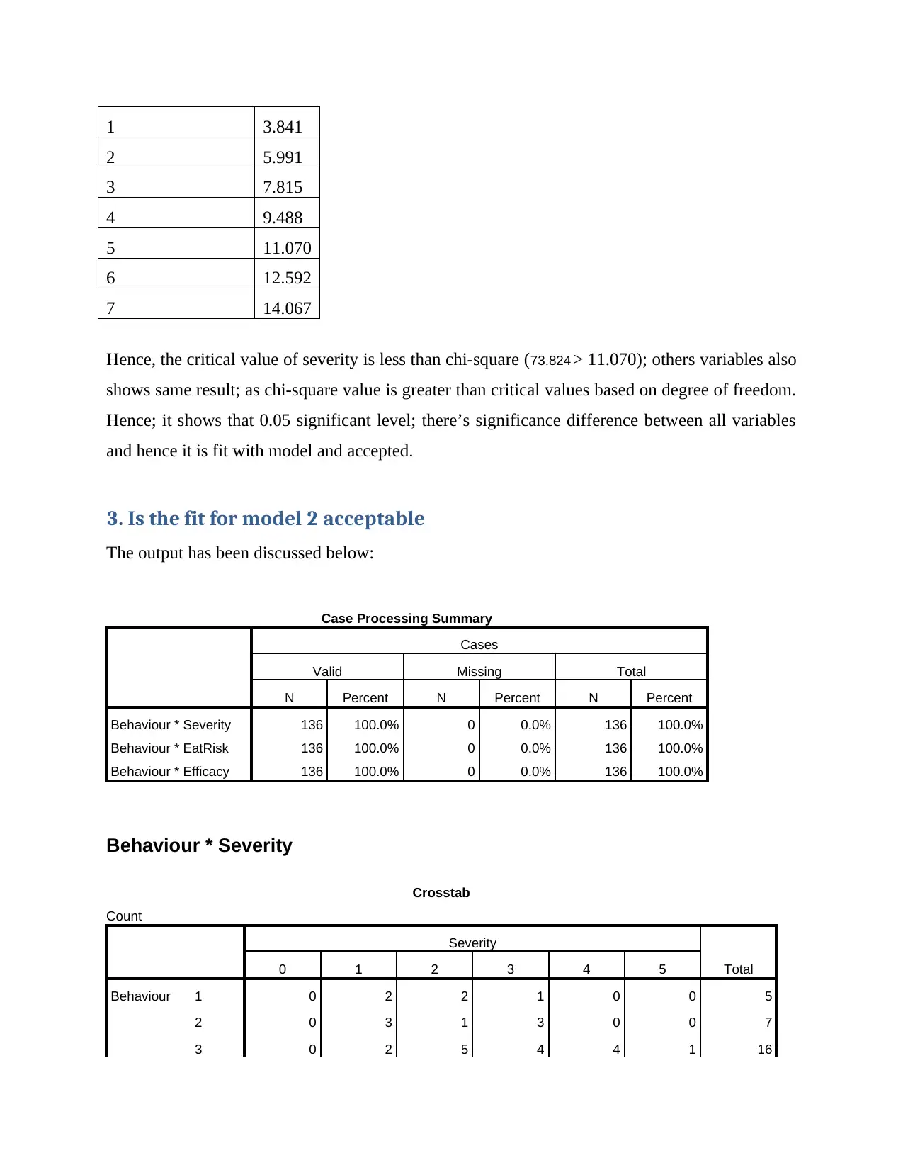
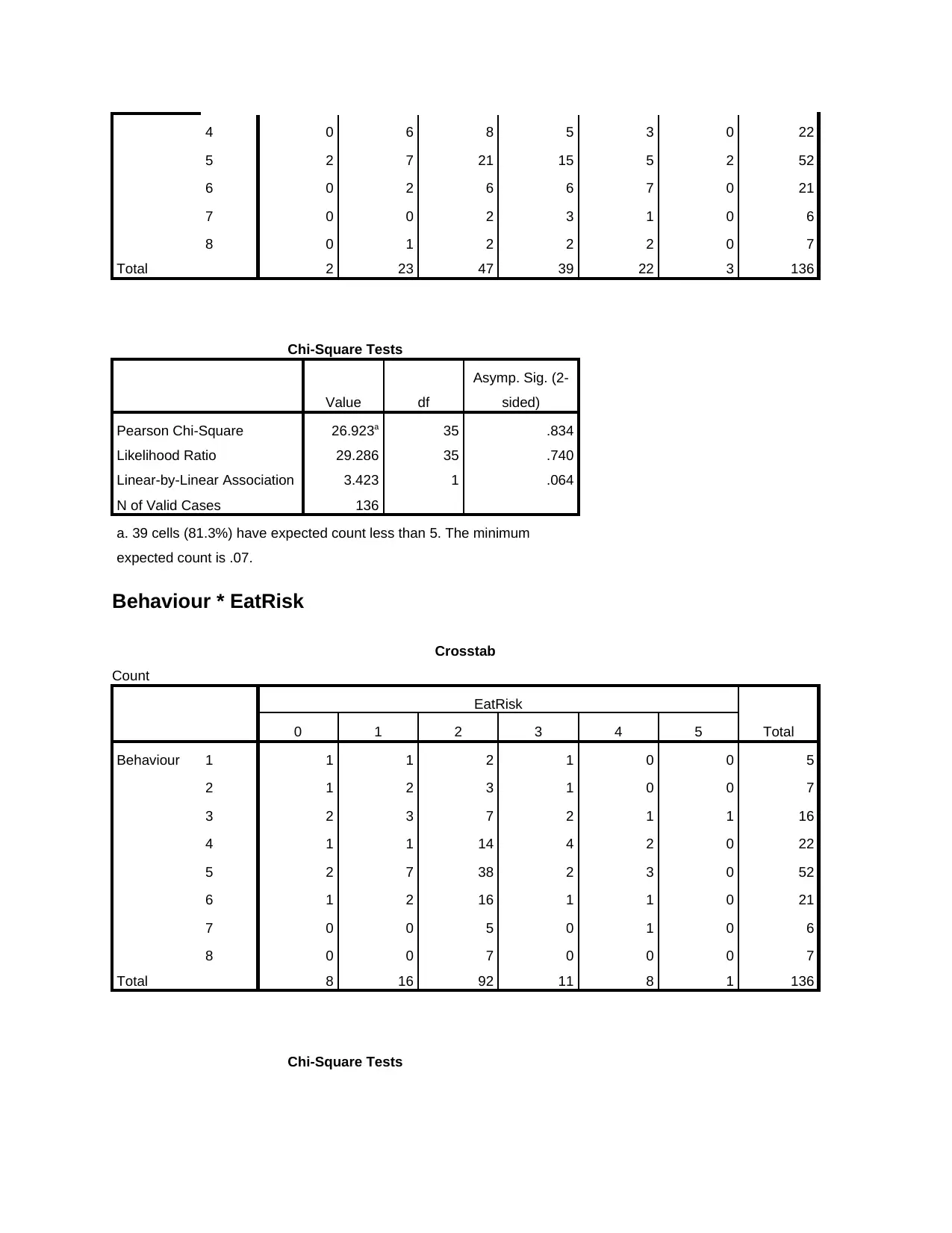
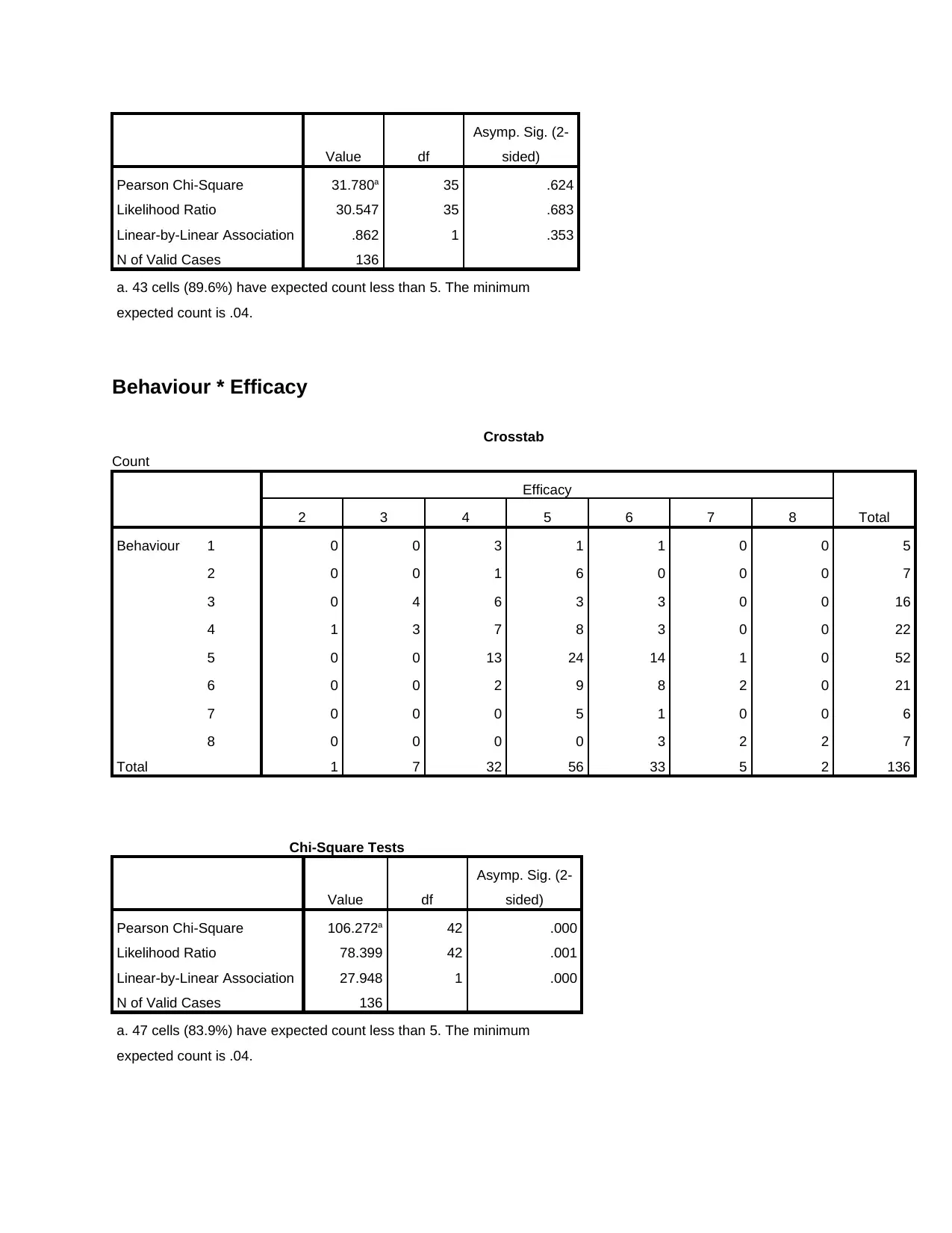
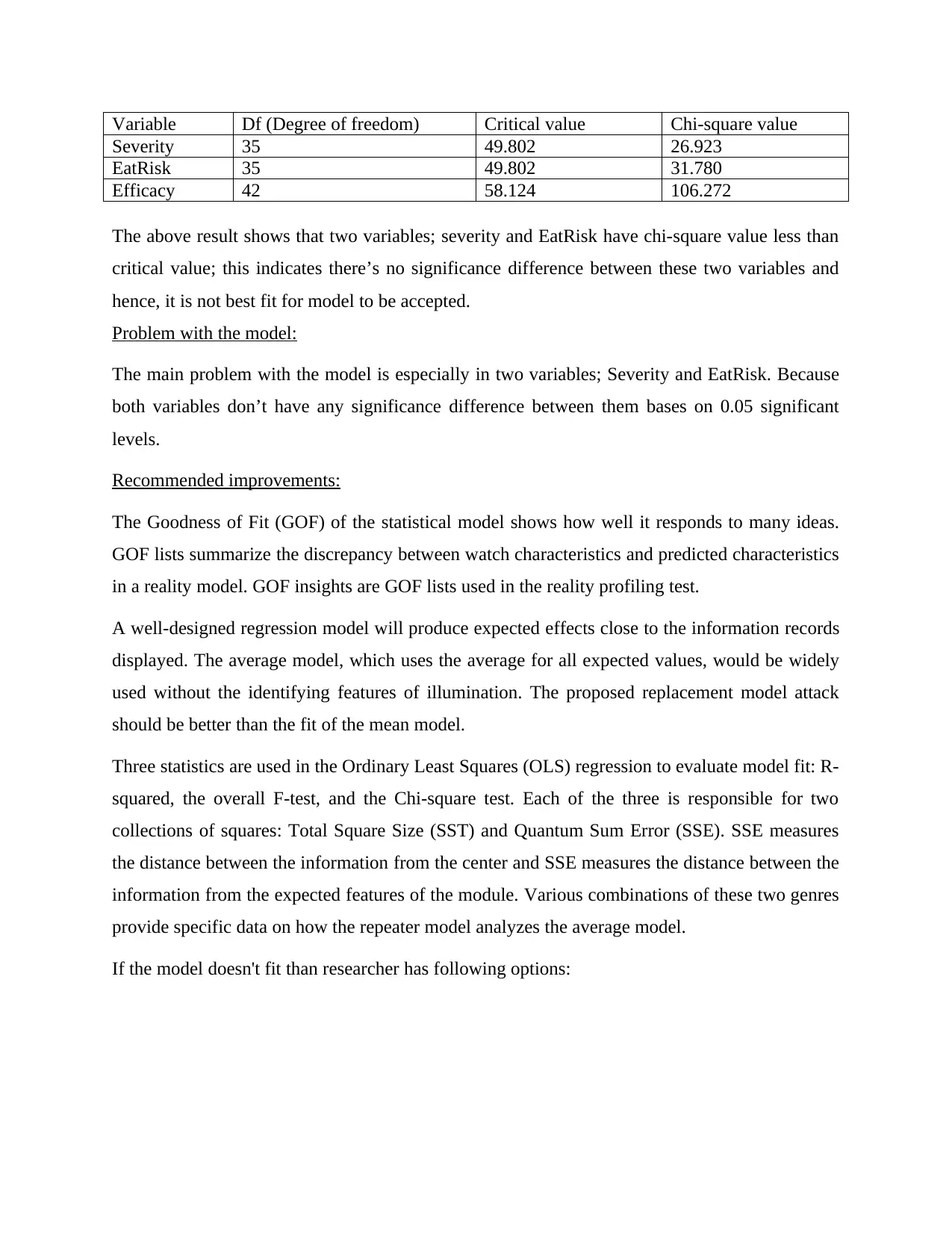
This assignment presents an analysis of two AMOS (Analysis of Moment Structures) models, focusing on their fit to the data and a comparison to determine which model is better. The analysis includes the evaluation of standardized path parameters for both models, followed by an assessment of the fit for each model using chi-square tests. The document details the chi-square test results for each variable in Model 1, including severity, EatRisk, GenRisk, and Conscious, and determines whether the fit is acceptable based on the critical values and degrees of freedom. Similarly, the analysis for Model 2 examines the fit based on chi-square tests for the relationships between Behavior and Severity, EatRisk, and Efficacy. The document identifies issues with Model 2, specifically highlighting that the chi-square values for Severity and EatRisk are less than critical values, indicating no significant difference. The assignment recommends improvements to the model, including the use of Goodness of Fit (GOF) statistics, and explores options for addressing model misfit. Finally, it concludes that Model 1 is the better fit based on the provided data and recommends its use for predicting behavior related to healthy eating.

AMOS analysis

1. Diagrams for Models 1 and 2 with standardized path parameters
Model 1:
Model 2
2. Is the fit for model 1 acceptable
To test whether fit for model 1 acceptable or not; chi-square has been used. Below is the output
of the test:
Severity
GenRisk
EatRisk Behavior
Conscious
-0.087 0.121
0.342
0.048
-.055
0.026
0.328
Severity
EatRisk
Efficacy
Behavior.000
-.228
0.131
0.492
0.158

Severity
Observed N Expected N Residual
0 2 22.7 -20.7
1 23 22.7 .3
2 47 22.7 24.3
3 39 22.7 16.3
4 22 22.7 -.7
5 3 22.7 -19.7
Total 136
EatRisk
Observed N Expected N Residual
0 8 22.7 -14.7
1 16 22.7 -6.7
2 92 22.7 69.3
3 11 22.7 -11.7
4 8 22.7 -14.7
5 1 22.7 -21.7
Total 136
GenRisk
Observed N Expected N Residual
2 36 34.0 2.0
3 76 34.0 42.0
4 20 34.0 -14.0
5 4 34.0 -30.0
Total 136

Conscious
Observed N Expected N Residual
2 2 22.7 -20.7
3 9 22.7 -13.7
4 34 22.7 11.3
5 49 22.7 26.3
6 34 22.7 11.3
7 8 22.7 -14.7
Total 136
Behaviour
Observed N Expected N Residual
1 5 17.0 -12.0
2 7 17.0 -10.0
3 16 17.0 -1.0
4 22 17.0 5.0
5 52 17.0 35.0
6 21 17.0 4.0
7 6 17.0 -11.0
8 7 17.0 -10.0
Total 136
Test Statistics
Severity EatRisk GenRisk Conscious Behaviour
Chi-Square 73.824a 259.735a 84.235b 78.500a 101.882c
df 5 5 3 5 7
Asymp. Sig. .000 .000 .000 .000 .000
a. 0 cells (0.0%) have expected frequencies less than 5. The minimum expected
cell frequency is 22.7.
b. 0 cells (0.0%) have expected frequencies less than 5. The minimum expected
cell frequency is 34.0.
c. 0 cells (0.0%) have expected frequencies less than 5. The minimum expected
cell frequency is 17.0.
Critical values:
Degrees of
freedom
0.05

1 3.841
2 5.991
3 7.815
4 9.488
5 11.070
6 12.592
7 14.067
Hence, the critical value of severity is less than chi-square (73.824 > 11.070); others variables also
shows same result; as chi-square value is greater than critical values based on degree of freedom.
Hence; it shows that 0.05 significant level; there’s significance difference between all variables
and hence it is fit with model and accepted.
3. Is the fit for model 2 acceptable
The output has been discussed below:
Case Processing Summary
Cases
Valid Missing Total
N Percent N Percent N Percent
Behaviour * Severity 136 100.0% 0 0.0% 136 100.0%
Behaviour * EatRisk 136 100.0% 0 0.0% 136 100.0%
Behaviour * Efficacy 136 100.0% 0 0.0% 136 100.0%
Behaviour * Severity
Crosstab
Count
Severity
Total0 1 2 3 4 5
Behaviour 1 0 2 2 1 0 0 5
2 0 3 1 3 0 0 7
3 0 2 5 4 4 1 16

4 0 6 8 5 3 0 22
5 2 7 21 15 5 2 52
6 0 2 6 6 7 0 21
7 0 0 2 3 1 0 6
8 0 1 2 2 2 0 7
Total 2 23 47 39 22 3 136
Chi-Square Tests
Value df
Asymp. Sig. (2-
sided)
Pearson Chi-Square 26.923a 35 .834
Likelihood Ratio 29.286 35 .740
Linear-by-Linear Association 3.423 1 .064
N of Valid Cases 136
a. 39 cells (81.3%) have expected count less than 5. The minimum
expected count is .07.
Behaviour * EatRisk
Crosstab
Count
EatRisk
Total0 1 2 3 4 5
Behaviour 1 1 1 2 1 0 0 5
2 1 2 3 1 0 0 7
3 2 3 7 2 1 1 16
4 1 1 14 4 2 0 22
5 2 7 38 2 3 0 52
6 1 2 16 1 1 0 21
7 0 0 5 0 1 0 6
8 0 0 7 0 0 0 7
Total 8 16 92 11 8 1 136
Chi-Square Tests

Value df
Asymp. Sig. (2-
sided)
Pearson Chi-Square 31.780a 35 .624
Likelihood Ratio 30.547 35 .683
Linear-by-Linear Association .862 1 .353
N of Valid Cases 136
a. 43 cells (89.6%) have expected count less than 5. The minimum
expected count is .04.
Behaviour * Efficacy
Crosstab
Count
Efficacy
Total2 3 4 5 6 7 8
Behaviour 1 0 0 3 1 1 0 0 5
2 0 0 1 6 0 0 0 7
3 0 4 6 3 3 0 0 16
4 1 3 7 8 3 0 0 22
5 0 0 13 24 14 1 0 52
6 0 0 2 9 8 2 0 21
7 0 0 0 5 1 0 0 6
8 0 0 0 0 3 2 2 7
Total 1 7 32 56 33 5 2 136
Chi-Square Tests
Value df
Asymp. Sig. (2-
sided)
Pearson Chi-Square 106.272a 42 .000
Likelihood Ratio 78.399 42 .001
Linear-by-Linear Association 27.948 1 .000
N of Valid Cases 136
a. 47 cells (83.9%) have expected count less than 5. The minimum
expected count is .04.

Variable Df (Degree of freedom) Critical value Chi-square value
Severity 35 49.802 26.923
EatRisk 35 49.802 31.780
Efficacy 42 58.124 106.272
The above result shows that two variables; severity and EatRisk have chi-square value less than
critical value; this indicates there’s no significance difference between these two variables and
hence, it is not best fit for model to be accepted.
Problem with the model:
The main problem with the model is especially in two variables; Severity and EatRisk. Because
both variables don’t have any significance difference between them bases on 0.05 significant
levels.
Recommended improvements:
The Goodness of Fit (GOF) of the statistical model shows how well it responds to many ideas.
GOF lists summarize the discrepancy between watch characteristics and predicted characteristics
in a reality model. GOF insights are GOF lists used in the reality profiling test.
A well-designed regression model will produce expected effects close to the information records
displayed. The average model, which uses the average for all expected values, would be widely
used without the identifying features of illumination. The proposed replacement model attack
should be better than the fit of the mean model.
Three statistics are used in the Ordinary Least Squares (OLS) regression to evaluate model fit: R-
squared, the overall F-test, and the Chi-square test. Each of the three is responsible for two
collections of squares: Total Square Size (SST) and Quantum Sum Error (SSE). SSE measures
the distance between the information from the center and SSE measures the distance between the
information from the expected features of the module. Various combinations of these two genres
provide specific data on how the repeater model analyzes the average model.
If the model doesn't fit than researcher has following options:

Reproduce a fragmentary evaluation of the model trying to decide the origin of the
nonconformist. This could be supported by modification files (e.g. Lagrange multiplication
baskets).
However, as they choose a model from the controversial options, they should struggle with
model misconduct. At the end of this, they can look at GOF records that penalize the
introduction of boundaries with, for example, AIC or BIC lists in the model. Alternatively, they
can plot the CFI chart, using the most important model under consideration as a benchmark.
Finally, when several factors are presented, it is unreasonable to expect a rigid model to respond
well - the overall dimensions of the test will be very large, as some parts of the information
around it will not be reproduced. with any stingy model.
Using a median of 5%, Chi-square and G-square suggest that the poor model should be accepted;
recommends the abolition of the model. Visualizations with a greater stimulus at the opportunity
level are generally more spectacular, and the results suggest greater strength squared M.
"Cell residues do not greatly support the piecemeal assessment of change. Specific residues (at a
rate of 5%) are captured for projects (10000), (01001) and (01000), which may suggest that can
be improve the attack of the model by releasing element 2. “The study of univariate and bivariate
remains offers another picture. Surprising remains can be found for (1,3), (1,5), (1,4) and (2,3),
which suggests that the non-controversial model is the result of object 1. This is certainly the
situation shown in a product, where Pearson's chi-square measurement was made after fall give
something at ac time.
Numerically speaking P (data) applies the scattering of P (theta), which in the typical Bayesian
way inflicts "punishment" for being too appropriate. Instead of choosing a theta that increases the
probability of P (data | theta) it is advisable to choose one that increases P (data | theta) P (theta).
Basically, this controls two different effects. The term P (data | theta) makes you choose a theta
that carefully models information, while the term P (theta) forces you to choose models that
naturally mean to be correct (as in the model I started with). These two neutralize each other and
the theta that governs them properly is usually flawless (thus avoiding too much change).

4. Which model is better
Based on the above output and discussion; it is found that model 1 is best fitted with the
available data and also better than model 2.
5. Summary
After analyzing all the data; it can be concluded that only one model (Model 1) is recommended
for predicting the behavior of people significance to the healthy eating; the main reason behind
this recommendation is acceptance of best fit model. As model 2; has not fitted due to less value
of Chi-square than critical value based on degree of freedom. This also indicates less variations
in the value of two variables of Model 2; EatRisk and Severity with the changes in the value of
Behavior.