UB Statistics Exam 1: Chapters 1-3 Analysis and Solutions

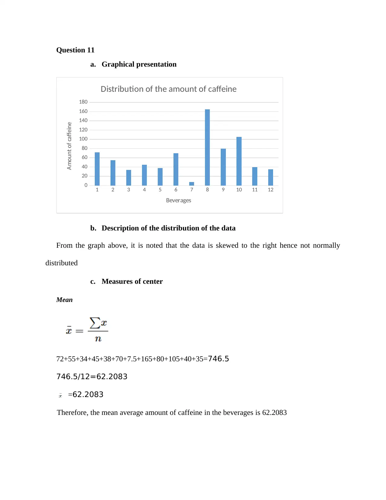
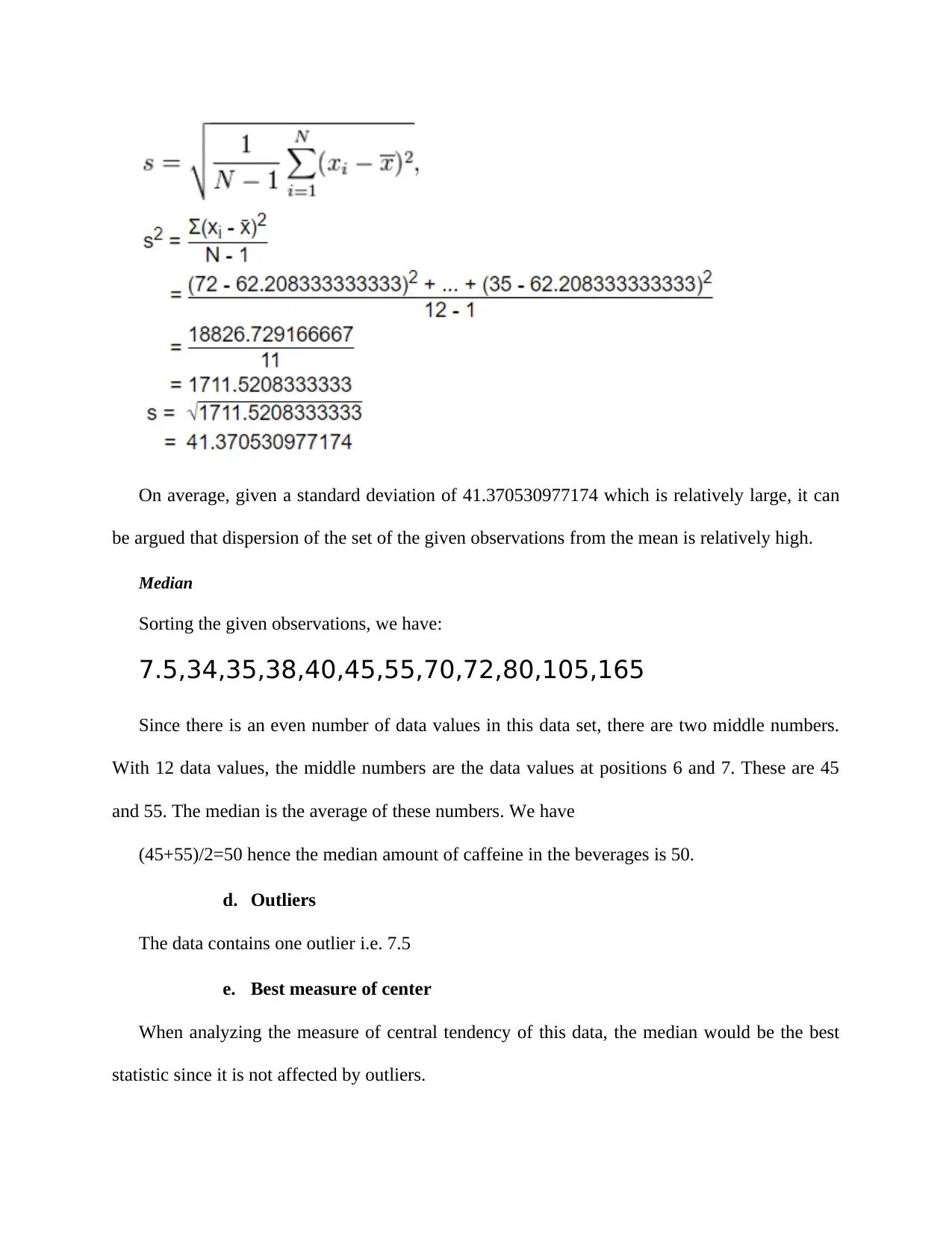
This document presents the solutions to a Statistics Exam 1, covering material from Chapters 1 through 3. The solutions include answers to multiple-choice questions and free-response problems. The free-response section involves analyzing a dataset of caffeine amounts in beverages. The analysis includes calculating the mean, median, and standard deviation; describing the data distribution; identifying outliers; determining the best measure of center; and calculating a z-score for a specific data point. The document also addresses sampling methods, including stratified random sampling, and estimation techniques for the mean number of discarded cans and bottles on public roads. The solutions are presented clearly, using statistical language and concepts.

Question 1
Only persons aged nineteen to thirty living in the state of Colorado
Question 2
The range in the amount of time in minutes’ males in the sample of customers spent in the
store is approximately 40 minutes.
Question 3
Cluster random sample
Question 4
The two cuts that are being roasted for each time-temperature combination are an example of
replication
Question 5
The mean is affected by the skewness whereas median is not
Question 6
The child will know whether he or she used flash cards or computer
Question 7
Stratified random sampling
Question 8
J, L, K
Question 9
Participants within each block should be as similar as possible with respect to how easily they
get sunburned.
Question 10
From the histogram it is noted that it is symmetric that is it has about the same shape on both
the right and left hence the data follows a normal distribution.

Question 11
a. Graphical presentation
1 2 3 4 5 6 7 8 9 10 11 12
0
20
40
60
80
100
120
140
160
180
Distribution of the amount of caffeine
Beverages
Amount of caffeine
b. Description of the distribution of the data
From the graph above, it is noted that the data is skewed to the right hence not normally
distributed
c. Measures of center
Mean
72+55+34+45+38+70+7.5+165+80+105+40+35=746.5
746.5/12=62.2083
=62.2083
Therefore, the mean average amount of caffeine in the beverages is 62.2083

On average, given a standard deviation of 41.370530977174 which is relatively large, it can
be argued that dispersion of the set of the given observations from the mean is relatively high.
Median
Sorting the given observations, we have:
7.5,34,35,38,40,45,55,70,72,80,105,165
Since there is an even number of data values in this data set, there are two middle numbers.
With 12 data values, the middle numbers are the data values at positions 6 and 7. These are 45
and 55. The median is the average of these numbers. We have
(45+55)/2=50 hence the median amount of caffeine in the beverages is 50.
d. Outliers
The data contains one outlier i.e. 7.5
e. Best measure of center
When analyzing the measure of central tendency of this data, the median would be the best
statistic since it is not affected by outliers.

f. Z score for the data point 45 mg/serving
The Z-score (z) is given by z = (x - μ) / σ
Where: x is the raw score value, μ is the mean of the population, σ is the standard deviation of
the population.
Hence:
x = 45, μ = 62.2083, σ = 41.370530977174
z = (45 - 62.2083) / 41.370530977174
z = -17.2083 / 41.370530977174 = -0.4160
Z-score for 45 mg/serving is -0.4160.
Question 12
a. The variable of Interest
The number of discarded cans and bottles in a one-mile segment of public road.
b. Parameter of interest
The mean number of discarded cans and bottles per mile of public road
c. Method of collection
The given data was collected using a stratified random sample. Especially given that the
agency divided the public roads into 3 categories on purpose then took a sample from each
category to form the collected sample.
d. Methods of estimating the mean
Ideally, method 1 provides a better estimate of this mean since it accounts for the relative
proportions of the number of miles for each type of roadway. On the other hand, method 2 treats
all the roadways equally despite the fact that there are differences in the number of miles for
each road type.