PACC6008: Statistical Analysis and Interpretation of Survey

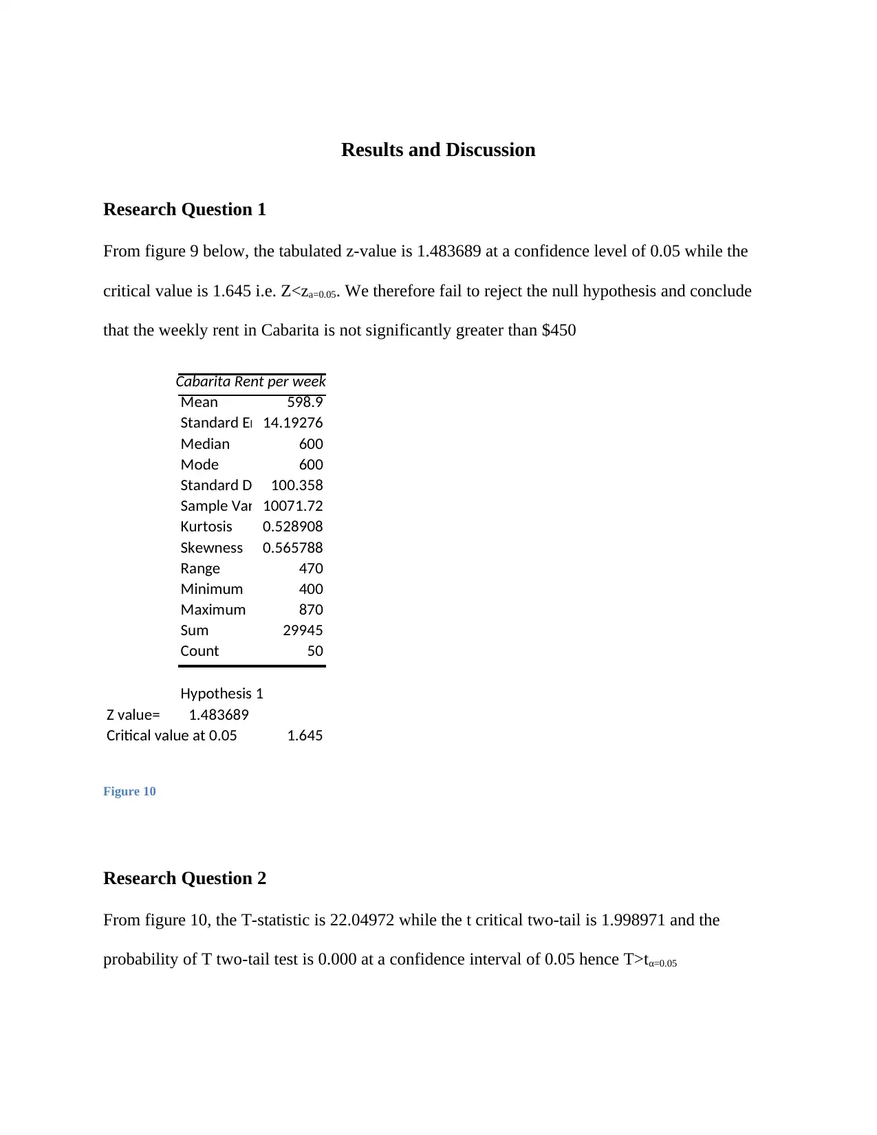
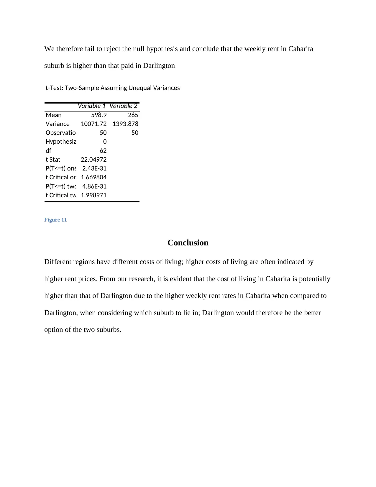
This assignment involves a statistical analysis of university survey data, focusing on GPA, child rank, and smoking habits among Australian university students. The analysis includes descriptive statistics and hypothesis testing using binomial, z, and t-tests. The binomial test is used to compare urban proportions, while z and t-tests are applied to analyze rental costs in Cabarita and Darlington, Sydney. The assignment concludes that there is no significant increase in the urban proportion of university students since 2017 and that the average weekly rent in Cabarita is higher than in Darlington. The document is available on Desklib, a platform offering study tools and resources for students.

Question 1
Part a
The population of interest is that of university going students in Australia.
Part b: Summary report
Following the analysis of: GPA, Child rank, and Smoker from the 2018 University survey, the
following results are deducted.
GPA
From figure 1, the average GPA mean of the 274 whose GPA information was available in the
sample population is 3.243051 with a standard deviation of 0.029442. The highest GPA scored
was 4, attained by 4 students whereas the least scored GPA is 1 attained by 1 student. Most of
the students have a GTPA of 3.4 i.e. 19 students followed by 16 students who recorded a GPA of
2.9.
GPA
Mean 3.243051
Standard Error0.029442
Median 3.3
Mode 3.4
Standard Deviation0.487344
Sample Variance0.237504
Kurtosis 2.178944
Skewness -1.0878
Range 3
Minimum 1
Maximum 4
Sum 888.596
Count 274
Figure 1: GPA Descriptive

Total
0
2
4
6
8
10
12
14
16
18
20
GPA1 1.3 1.4 2 2.2 2.3
2.336 2.4 2.5 2.57 2.6 2.66
2.7 2.75 2.8 2.89 2.9 2.911
2.95 2.97 2.987 3 3.007 3.05
3.065 3.07 3.1 3.101 3.138 3.15
3.189 3.2 3.212 3.22 3.223 3.24
3.241 3.25 3.26 3.268 3.28 3.3
3.301 3.315 3.32 3.33 3.34 3.36
3.37 3.4 3.43 3.441 3.45 3.46
3.47 3.471 3.48 3.488 3.49 3.5
3.53 3.535 3.54 3.541 3.55 3.556
3.56 3.57 3.58 3.59 3.6 3.614
3.63 3.632 3.65 3.655 3.67 3.68
3.692 3.7 3.72 3.724 3.738 3.75
3.76 3.78 3.8 3.83 3.84 3.85
3.87 3.872 3.875 3.9 3.902 3.906
3.908 3.91 3.94 3.994 4 (blank)
Figure 2: GPA
Child rank
Most students in the sample are first born, i.e. 88 whereas those in the 2nd rank are 82, those in
the 3rd are 67, in the 4th are 27 while those in the 5th, 6th, and 7th are 13, 2, and 1 respectively.
childrank
Mean 2.303571
Standard Error0.072551
Median 2
Mode 1
Standard Deviation1.214011
Sample Variance1.473822
Kurtosis 0.408978
Skewness 0.840714
Range 6
Minimum 1
Maximum 7
Sum 645
Count 280
Figure 3: Child Rank Descriptive

1
3
5
7
9
11
13
15
17
19
21
23
25
27
29
31
33
35
37
0
1
2
3
4
5
6
7
8
childrank
childrank
Figure 4: Child Rank
Smoker
Row Labels Count of smoker
Non 258
Smoke 18
(blank)
Grand Total 276
Figure 5: Smoker Descriptive
From figure 5 above, the total number of non-smokers in the sample data is 258 while there are
18 smokers

Total
0
50
100
150
200
250
300
Smoker
Non
Smoke
(blank)
Figure 6: Smoker
Part C
Introduction
Appropriate test
Since we wish to compare different proportions of the same population, i.e. measure proportional
performance, the appropriate test is the Binomial test
Hypotheses
Null Hypothesis
The urban proportion in the population in 2018 is less than or equal to that of 2017, i.e. H0:
p≤0.15
Alternative Hypothesis
The urban proportion in the population in 2018 is greater than that of 2017, i.e. H1: p> 0.15.
Methodology
Following our null hypothesis, we apply a one-tailed test using the pre-stated null and alternative
hypothesis. In Excel we use:

Hence p-value=1-BinomDist (n, p, 1-α)
Where n=38, p=280, α=0.05
Results
Null: p≤0.15
Alt: p>0.15
n=38
p=280
p-value=1-BINOM>DIST(38,280, .15, TRUE)
p-value= 0.944828
Figure 7
From figure 7 above, the p-value is 0.944828 which is greater than 0.05 such that P>pα=0.05.
Prompting that we fail to reject the null hypothesis (Real statistics, 2018) and conclude that there
is no enough statistical evidence that the urban proportion in the population survey of 2018
significantly increased since 2017.
Conclusion
In conclusion, binomial tests are used in testing hypothesis involving population proportions
such as the preceding one. In our study of interest we can therefore deduct that it is true the urban
population among university students has remained relatively the same or has dropped from the
year 2018.

Question 2
Report
Introduction
The adage that equates one’s home to one’s castle cannot be truer given the current need for
proper housing; hence, when looking out for places to live, it is often crucial to put into
consideration a number of issues such as security, comfort, access to essential services and most
importantly cost. In this study, we will employ statistical tests to compare the cost of renting a
two bedroom apartment in Cabarita and Darlington, suburbs in Sydney so as to aid in making the
optimal choice as to which suburb to live in under optimal conditions.
Research Questions
1. Is the average rent in Cabarita significantly greater than 450?
2. Is the average rent in Cabarita higher than that in Darlington

Methodology
Data
The dataset for this study is obtained from Australian real estate website www.realestate.com.au
under Cabarita and Darlington sub topics.
Data Demography
Rent per week In Darlington
Mean 265
Standard Error5.27992
Median 250
Mode 250
Standard Deviation37.33467
Sample Variance1393.878
Kurtosis -0.77034
Skewness 0.497864
Range 135
Minimum 210
Maximum 345
Sum 13250
Count 50
Figure 8
The average rent per week in Darlington is $265 (fig 7). The total sample size is 50 and the
standard deviation is $37.33467 while the most paid rent per week is $250

Cabarita Rent per week
Mean 598.9
Standard Error14.19276
Median 600
Mode 600
Standard Deviation100.358
Sample Variance10071.72
Kurtosis 0.528908
Skewness 0.565788
Range 470
Minimum 400
Maximum 870
Sum 29945
Count 50
Figure 9
The average rent in Cabarita is $598.9 (fig 8). The total sample size is 50 and the standard
deviation is $100.358 while the most paid rent is $600.
Hypotheses
Null hypothesis 1
H0: The average weekly rent in Cabarita is significantly greater than 450 i.e. H0: μ> 450
Alternative hypothesis 1
H1: The average weekly rent in Cabarita is not significantly greater than 450 i.e. H1: μ≠> 450
In the current form, we seek to compare a composite null hypothesis against a composite
alternative hypothesis. We convert the null and alternative hypotheses into simple against simple
hypothesis such that:
H0: (μ=μ0: μ0>450)
H1: (μ=μ1: μ1≠>450)
Null hypothesis 2
H0: The average weekly rent in Cabarita is greater than that of Darlington i.e. H0: μ0> μ1

Alternative hypothesis 2
H1: The average weekly rent in Cabarita is not greater than that of Darlington i.e. H0: μ0< μ1
Process
In the first set of hypotheses, we seek to test the hypothesis around the sample mean where the
standard deviation and population mean are known. We therefore use the Z-test (Mann, 2012):
Z=
X−μ
σ
√ n
where n is the sample size, σ is the S.D and X the sample mean. We reject the null
hypothesis is p(Z<α=0.05) (Sullivan, 2015).
In the second set of hypothesis, we use the t-test since we are testing the null hypothesis that the
average weekly cost of Darlington and Cabarita are equal (Deborah, 2017), i.e.:
T=
X 1− X 2
√ S 12
N 1 −¿ S 22
N 2 ¿

Results and Discussion
Research Question 1
From figure 9 below, the tabulated z-value is 1.483689 at a confidence level of 0.05 while the
critical value is 1.645 i.e. Z<za=0.05. We therefore fail to reject the null hypothesis and conclude
that the weekly rent in Cabarita is not significantly greater than $450
Cabarita Rent per week
Mean 598.9
Standard Error14.19276
Median 600
Mode 600
Standard Deviation100.358
Sample Variance10071.72
Kurtosis 0.528908
Skewness 0.565788
Range 470
Minimum 400
Maximum 870
Sum 29945
Count 50
Hypothesis 1
Z value= 1.483689
Critical value at 0.05 1.645
Figure 10
Research Question 2
From figure 10, the T-statistic is 22.04972 while the t critical two-tail is 1.998971 and the
probability of T two-tail test is 0.000 at a confidence interval of 0.05 hence T>tα=0.05

We therefore fail to reject the null hypothesis and conclude that the weekly rent in Cabarita
suburb is higher than that paid in Darlington
t-Test: Two-Sample Assuming Unequal Variances
Variable 1 Variable 2
Mean 598.9 265
Variance 10071.72 1393.878
Observations 50 50
Hypothesized Mean Difference0
df 62
t Stat 22.04972
P(T<=t) one-tail2.43E-31
t Critical one-tail1.669804
P(T<=t) two-tail4.86E-31
t Critical two-tail1.998971
Figure 11
Conclusion
Different regions have different costs of living; higher costs of living are often indicated by
higher rent prices. From our research, it is evident that the cost of living in Cabarita is potentially
higher than that of Darlington due to the higher weekly rent rates in Cabarita when compared to
Darlington, when considering which suburb to lie in; Darlington would therefore be the better
option of the two suburbs.

Bibliography
Deborah, J.R. (2017). How to compare two population proportions. Retrieved from:
https://www.dummies.com/education/math/statistics/how-to-compare-two-population-
proportions/
Mann, P. (2012). Estimation of the Mean and Proportion: A statistics paper. Excel essentials,
23(12), 33-35
NCSS. (2013). Tests for one proportion. NCSS, LLC :Author
Real Statistics. (2018). Real Statistics using Excel. Retrieved from:
www.real-statistics.com/binomial-and-related-distributions/hypothesis-testing-binomial-
distribution/
Sullivan, L. (2015). Hypothesis Testing for Means & Proportions. Retrieved from:
http://sphweb.bumc.bu.edu/otlt/MPH-Modules/BS/BS704_HypothesisTest-Means-
Proportions/BS704_HypothesisTest-Means-Proportions_print.html