University Quantitative Methods Assignment Analysis Report

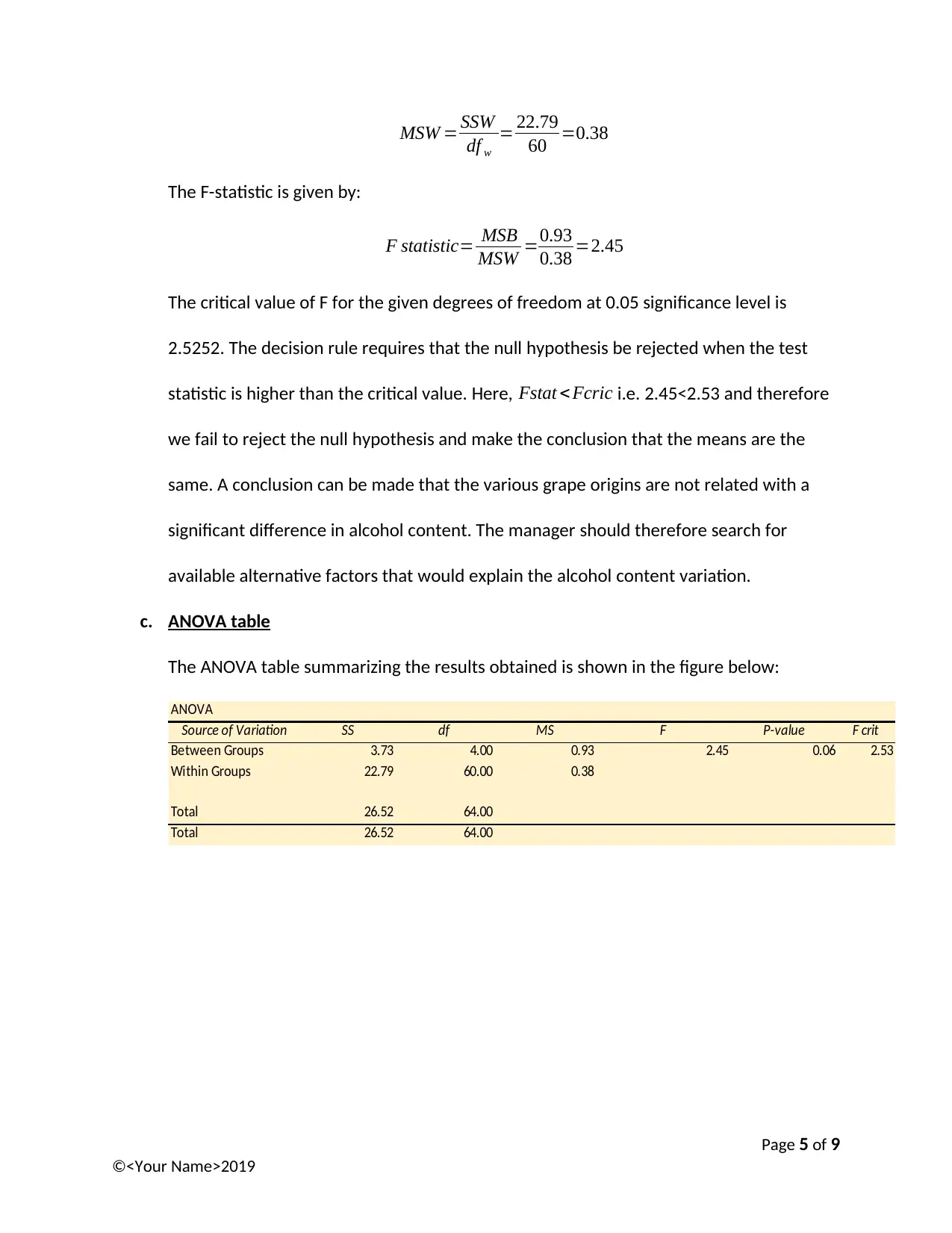
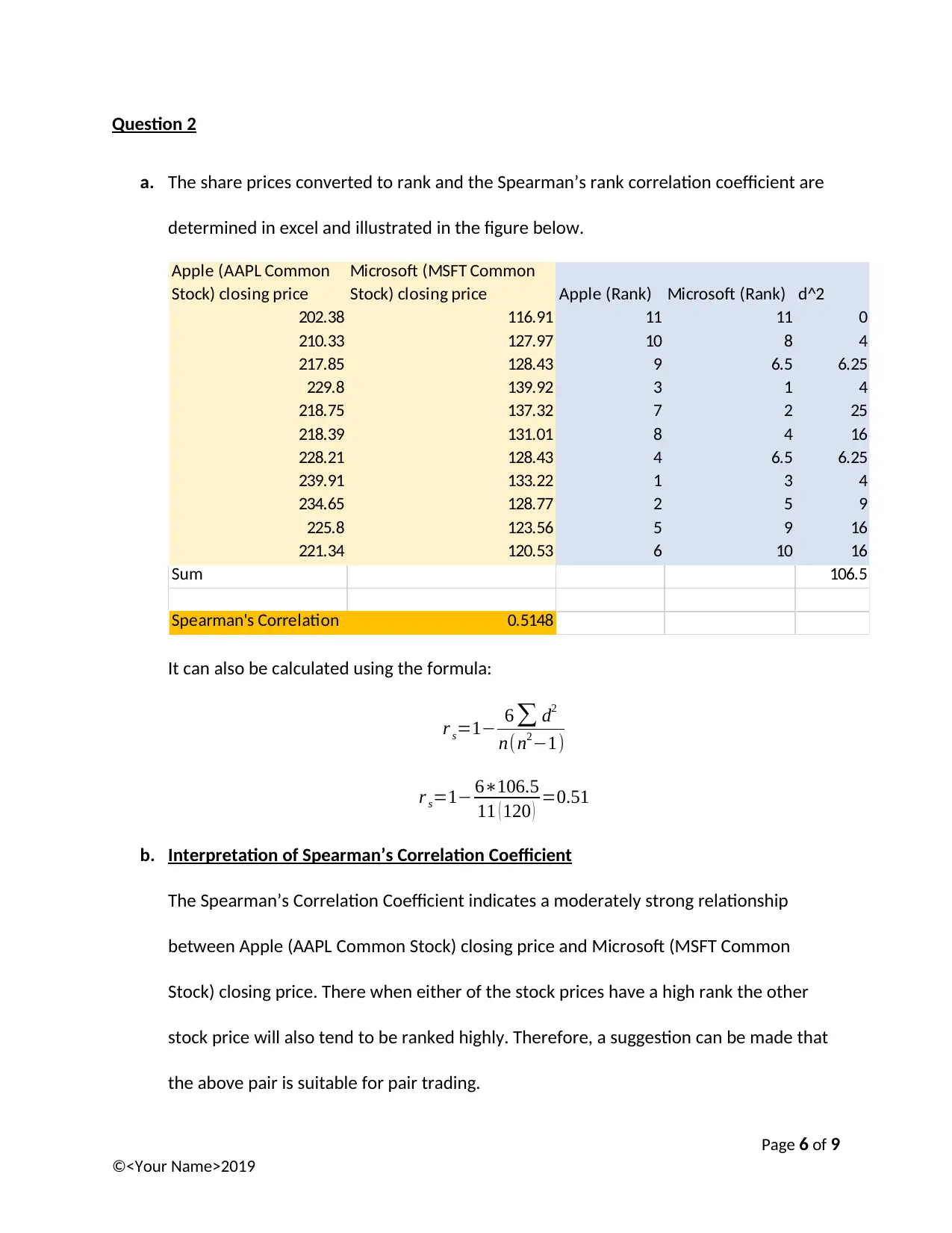
This document presents a comprehensive solution to a Quantitative Methods assignment, addressing a scenario involving a winery and its Pinot Noir production. The assignment involves analyzing the variation in alcohol content based on the origin of grapes. The solution includes an ANOVA test to determine if there are significant differences in alcohol content among different grape origins. It also explores Spearman's rank correlation to assess the relationship between the closing prices of two stocks, Apple and Microsoft, and performs a hypothesis test to determine the significance of the correlation. Furthermore, the document discusses Type I and Type II errors in the context of statistical analysis, providing clear explanations and examples. The assignment demonstrates the application of statistical methods to real-world business problems, offering insights into data analysis and decision-making. The document is a valuable resource for students seeking to understand and solve quantitative problems.

University
Quantitative Methods
By
Your Name
Date
Page 1 of 9
©<Your Name>2019

Quantitative Methods
Question 1
a. Column Scatter Plot
The green lines shown the variation within the groups.
The blue lines show the variation between the groups
The orange line shows the group mean
The short black lines show the individual means of each group.
Page 2 of 9
©<Your Name>2019

b. Test for Independence
The data to be used is shown in the table below.
Estate Southern Ridge Wine Valley Maisie and Co Kate's Corner
11.31 11.15 10.63 11.78 11.58
11.98 12.80 11.62 12.98 12.47
11.89 12.25 11.66 11.90 12.51
12.39 11.81 11.03 12.48 11.47
12.34 12.03 12.67 13.36 12.72
13.02 12.35 12.70 12.47 12.01
12.61 12.59 13.31 12.82 12.71
11.69 12.89 12.76 12.41 12.03
12.59 12.23 11.64 13.04 12.80
11.54 12.52 12.36 12.39 12.09
12.38 12.13 12.25 12.68 12.46
11.43 11.09 10.64 11.96 11.62
12.13 12.26 11.86 14.16 12.02
∑x 157.3 158.1 155.13 164.43 158.49
∑x^2 1906.51 1926.36 1859.62 2084.84 1934.73
Average 12.10 12.16 11.93 12.65 12.19
SS 3.18 3.62 8.44 5.06 2.49
The null and the alternative hypothesis are stated as:
Null hypothesis Ho : μ1=μ2=μ3=μ4 =μ5
Alternative hypothesis Hi :μ1 ≠ μ2 ≠ μ3 ≠ μ4=μ5
The assumption made is that each of the variables has the same variance.
The sample size n=13 while the number of groups a=5
The degrees of freedom:
df t =df B +df w
Degrees of freedom between groups:
df B=Ngroups−1
df B=5−1=4
The degrees of freedom between groups:
Page 3 of 9
©<Your Name>2019

df w=N−Ngroups
df w=65−5=60
Total degrees of freedom:
df t =60+ 4=64 d f
The combined mean of the groups is given by:
M = ( μ1+ μ2 +μ3 +μ4 + μ5
Ngroups )
GM =( 12.10+12.16+11.93+12.65+12.19
5 )=12.21
The variability between groups:
SSB=n1 {( μ1−GM )
2 + ( μ2 −GM )
2 + ( μ3 −GM )
2 + ( μ4−GM )
2+ ( μ5−GM ) 2 }
SSB=13(0.0121+ 0.0025+0.0784+0.1936+0.0004)
SSB=3.731
The variability within groups is:
SSW =SS 1+ SS 2+ SS 3+ SS 4+SS 5
SSW =3.18+3.62+8.44+5.06+2.49
SSW =22. 7 9
Sum of squares:
SST =SSB+SSW
SST =3.731+ 22.79=26.5 2
The mean square between groups:
MSB= SSB
df b
= 3.731
4 =0.93
The mean square within groups
Page 4 of 9
©<Your Name>2019

MSW = SSW
df w
= 22.79
60 =0.38
The F-statistic is given by:
F statistic= MSB
MSW =0.93
0.38 =2.45
The critical value of F for the given degrees of freedom at 0.05 significance level is
2.5252. The decision rule requires that the null hypothesis be rejected when the test
statistic is higher than the critical value. Here, Fstat < Fcric i.e. 2.45<2.53 and therefore
we fail to reject the null hypothesis and make the conclusion that the means are the
same. A conclusion can be made that the various grape origins are not related with a
significant difference in alcohol content. The manager should therefore search for
available alternative factors that would explain the alcohol content variation.
c. ANOVA table
The ANOVA table summarizing the results obtained is shown in the figure below:
ANOVA
Source of Variation SS df MS F P-value F crit
Between Groups 3.73 4.00 0.93 2.45 0.06 2.53
Within Groups 22.79 60.00 0.38
Total 26.52 64.00
Total 26.52 64.00
Page 5 of 9
©<Your Name>2019

Question 2
a. The share prices converted to rank and the Spearman’s rank correlation coefficient are
determined in excel and illustrated in the figure below.
Apple (AAPL Common
Stock) closing price
Microsoft (MSFT Common
Stock) closing price Apple (Rank) Microsoft (Rank) d^2
202.38 116.91 11 11 0
210.33 127.97 10 8 4
217.85 128.43 9 6.5 6.25
229.8 139.92 3 1 4
218.75 137.32 7 2 25
218.39 131.01 8 4 16
228.21 128.43 4 6.5 6.25
239.91 133.22 1 3 4
234.65 128.77 2 5 9
225.8 123.56 5 9 16
221.34 120.53 6 10 16
Sum 106.5
Spearman's Correlation 0.5148
It can also be calculated using the formula:
r s=1− 6 ∑ d2
n(n2−1)
r s=1− 6∗106.5
11 ( 120 ) =0.51
b. Interpretation of Spearman’s Correlation Coefficient
The Spearman’s Correlation Coefficient indicates a moderately strong relationship
between Apple (AAPL Common Stock) closing price and Microsoft (MSFT Common
Stock) closing price. There when either of the stock prices have a high rank the other
stock price will also tend to be ranked highly. Therefore, a suggestion can be made that
the above pair is suitable for pair trading.
Page 6 of 9
©<Your Name>2019

c. Hypothesis Test
The null and alternative hypothesis are stated as:
Null hypothesis Ho : ρs ≥ 0.6
The alternative hypothesis Hi : ρs <0.6
This is a one tailed test with alpha equals to 0.05, n= 11 and the Spearman’s correlation
coefficient equals to 0.5148.
The test statistic is determined by:
z= rs −ρs
σr s
Where:
σ rs
= 1
√ ( n−1 ) = 1
√ 10 =0.31623
Hence:
z= 0.5148−0.6
0.31623 =−0.2694
The critical value of z is:
Zcrit=± Z0.05=± 1.64
The test statistics obtained is -0.07 and therefore it false with the bound of the critical
values. From the decision rule, we fail to reject the null hypothesis and make a
conclusion that with a 5% significance level the investor is supposed to seek for a full
year data (Evans and Basu, 2013).
d. Type 1 and Type II error
A type I error is a statistical error that occurs when a true null hypothesis is rejected. For
example, in our case, we concluded that the correlation in the population was not
Page 7 of 9
©<Your Name>2019

strong ρs< 0.6 we would have committed a type I error since the relationship is actually
strong.
Type II error occurs is a statistical error that occurs when we fail to reject a false null
hypothesis (Watkins, Scheaffer, and Cobb, 2009). For example, in this case, type II error
would occur if we concluded that there is a strong correlation between the variables
ρs ≥ 0.6when in reality there is no strong relationship.
Page 8 of 9
©<Your Name>2019

References
Evans, J. R., and Basu, A. 2013. Statistics, data analysis, and decision modeling.5th ed. Boston:
Pearson.
Watkins, A. E., Scheaffer, R. L., and Cobb, G. W. 2009. Statistics in action: Understanding a
world of data. 2nd ed. Hoboken, NJ: Wiley
Page 9 of 9
©<Your Name>2019