Detailed Statistics and Probability Assignment for University Students
VerifiedAdded on 2022/09/23
|12
|1857
|40
Homework Assignment
AI Summary
This document presents a comprehensive solution to a post-module statistics assignment. The assignment encompasses various statistical concepts, including independent samples t-tests, hypothesis testing, and probability distributions such as Poisson distribution. It addresses questions related to comparing sales data across different areas, analyzing the relationship between sales and floor space, and calculating confidence intervals. The solution also involves analyzing data from experiments, such as the impact of ingredients on the strength of bonded sand moulds and the effect of alcohol on reaction time. Moreover, the assignment covers topics like modeling breakdown occurrences, comparing median values, and calculating probabilities related to defects in manufacturing processes and repair times. Statistical software output is used to support the analysis and the assumptions behind each statistical test are highlighted.
1
POST MODULE ASSIGNMENT
DEADLINE:
To be submitted electronically BEFORE 12:00 noon UK time on 12/04/2020
NB: Late submission of coursework without approval for an extension will result in marks being deducted
up to a maximum of 10 University working days late. After this period, the work may be counted as a non-
submission.
Paraphrase This Document
Need a fresh take? Get an instant paraphrase of this document with our AI Paraphraser
2
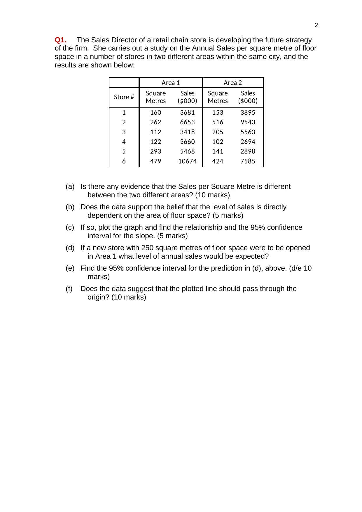
Q1. The Sales Director of a retail chain store is developing the future strategy
of the firm. She carries out a study on the Annual Sales per square metre of floor
space in a number of stores in two different areas within the same city, and the
results are shown below:
Area 1 Area 2
Store #
1 160 3681 153 3895
2 262 6653 516 9543
3 112 3418 205 5563
4 122 3660 102 2694
5 293 5468 141 2898
6 479 10674 424 7585
Square
Metres
Sales
($000)
Square
Metres
Sales
($000)
(a) Is there any evidence that the Sales per Square Metre is different
between the two different areas? (10 marks)
(b) Does the data support the belief that the level of sales is directly
dependent on the area of floor space? (5 marks)
(c) If so, plot the graph and find the relationship and the 95% confidence
interval for the slope. (5 marks)
(d) If a new store with 250 square metres of floor space were to be opened
in Area 1 what level of annual sales would be expected?
(e) Find the 95% confidence interval for the prediction in (d), above. (d/e 10
marks)
(f) Does the data suggest that the plotted line should pass through the
origin? (10 marks)
3
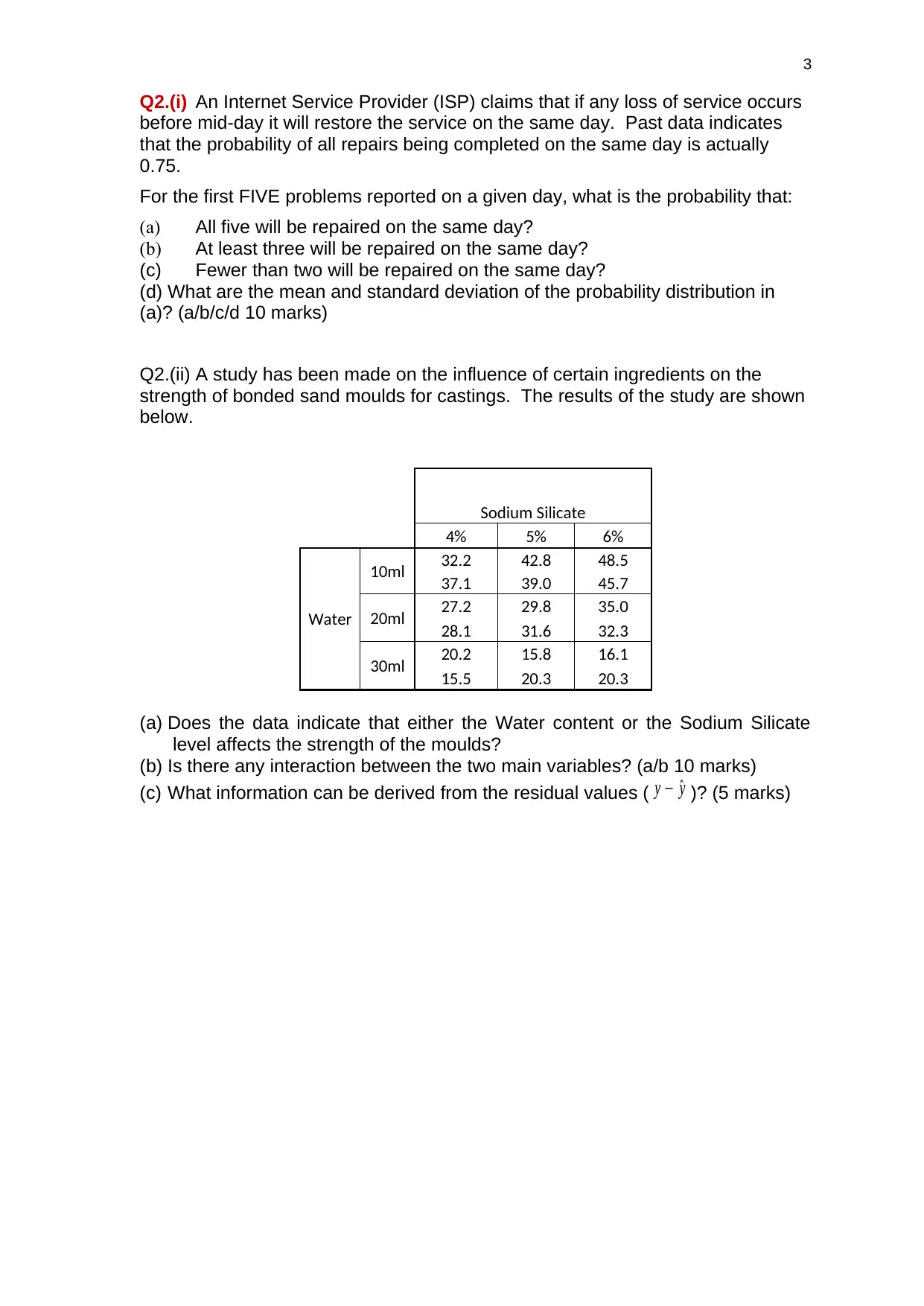
Q2.(i) An Internet Service Provider (ISP) claims that if any loss of service occurs
before mid-day it will restore the service on the same day. Past data indicates
that the probability of all repairs being completed on the same day is actually
0.75.
For the first FIVE problems reported on a given day, what is the probability that:
(a) All five will be repaired on the same day?
(b) At least three will be repaired on the same day?
(c) Fewer than two will be repaired on the same day?
(d) What are the mean and standard deviation of the probability distribution in
(a)? (a/b/c/d 10 marks)
Q2.(ii) A study has been made on the influence of certain ingredients on the
strength of bonded sand moulds for castings. The results of the study are shown
below.
Sodium Silicate
4% 5% 6%
Water
10ml 32.2 42.8 48.5
37.1 39.0 45.7
20ml 27.2 29.8 35.0
28.1 31.6 32.3
30ml 20.2 15.8 16.1
15.5 20.3 20.3
(a) Does the data indicate that either the Water content or the Sodium Silicate
level affects the strength of the moulds?
(b) Is there any interaction between the two main variables? (a/b 10 marks)
(c) What information can be derived from the residual values ( y − ^y )? (5 marks)
⊘ This is a preview!⊘
Do you want full access?
Subscribe today to unlock all pages.
Trusted by 1+ million students worldwide
4
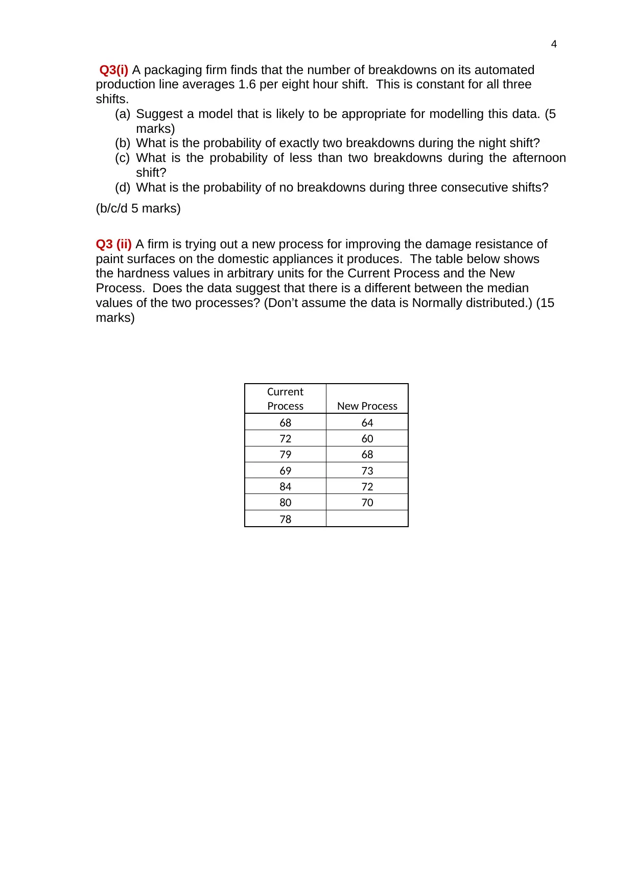
Q3(i) A packaging firm finds that the number of breakdowns on its automated
production line averages 1.6 per eight hour shift. This is constant for all three
shifts.
(a) Suggest a model that is likely to be appropriate for modelling this data. (5
marks)
(b) What is the probability of exactly two breakdowns during the night shift?
(c) What is the probability of less than two breakdowns during the afternoon
shift?
(d) What is the probability of no breakdowns during three consecutive shifts?
(b/c/d 5 marks)
Q3 (ii) A firm is trying out a new process for improving the damage resistance of
paint surfaces on the domestic appliances it produces. The table below shows
the hardness values in arbitrary units for the Current Process and the New
Process. Does the data suggest that there is a different between the median
values of the two processes? (Don’t assume the data is Normally distributed.) (15
marks)
Current
Process New Process
68 64
72 60
79 68
69 73
84 72
80 70
78
Paraphrase This Document
Need a fresh take? Get an instant paraphrase of this document with our AI Paraphraser
5
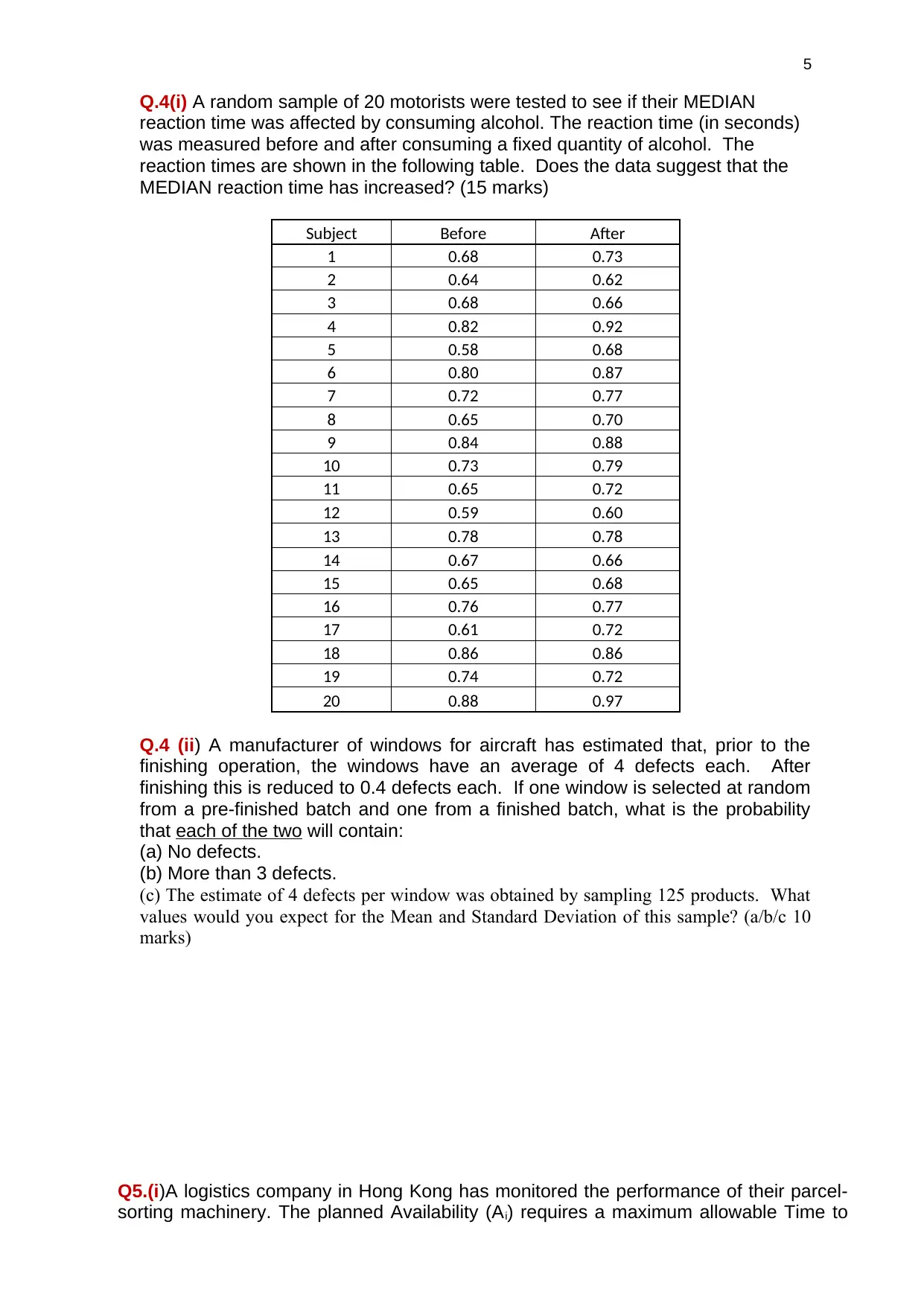
Q.4(i) A random sample of 20 motorists were tested to see if their MEDIAN
reaction time was affected by consuming alcohol. The reaction time (in seconds)
was measured before and after consuming a fixed quantity of alcohol. The
reaction times are shown in the following table. Does the data suggest that the
MEDIAN reaction time has increased? (15 marks)
Subject Before After
1 0.68 0.73
2 0.64 0.62
3 0.68 0.66
4 0.82 0.92
5 0.58 0.68
6 0.80 0.87
7 0.72 0.77
8 0.65 0.70
9 0.84 0.88
10 0.73 0.79
11 0.65 0.72
12 0.59 0.60
13 0.78 0.78
14 0.67 0.66
15 0.65 0.68
16 0.76 0.77
17 0.61 0.72
18 0.86 0.86
19 0.74 0.72
20 0.88 0.97
Q.4 (ii) A manufacturer of windows for aircraft has estimated that, prior to the
finishing operation, the windows have an average of 4 defects each. After
finishing this is reduced to 0.4 defects each. If one window is selected at random
from a pre-finished batch and one from a finished batch, what is the probability
that each of the two will contain:
(a) No defects.
(b) More than 3 defects.
(c) The estimate of 4 defects per window was obtained by sampling 125 products. What
values would you expect for the Mean and Standard Deviation of this sample? (a/b/c 10
marks)
Q5.(i)A logistics company in Hong Kong has monitored the performance of their parcel-
sorting machinery. The planned Availability (Ai) requires a maximum allowable Time to
6
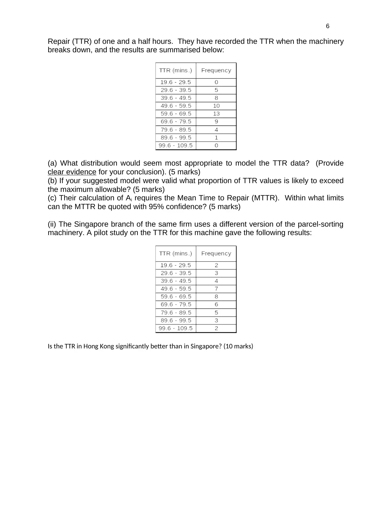
Repair (TTR) of one and a half hours. They have recorded the TTR when the machinery
breaks down, and the results are summarised below:
(a) What distribution would seem most appropriate to model the TTR data? (Provide
clear evidence for your conclusion). (5 marks)
(b) If your suggested model were valid what proportion of TTR values is likely to exceed
the maximum allowable? (5 marks)
(c) Their calculation of Ai requires the Mean Time to Repair (MTTR). Within what limits
can the MTTR be quoted with 95% confidence? (5 marks)
(ii) The Singapore branch of the same firm uses a different version of the parcel-sorting
machinery. A pilot study on the TTR for this machine gave the following results:
Is the TTR in Hong Kong significantly better than in Singapore? (10 marks)
⊘ This is a preview!⊘
Do you want full access?
Subscribe today to unlock all pages.
Trusted by 1+ million students worldwide
7
MODULE TITLE
Table of Contents
1 Independent samples t-test..................................................................................................... 8
2 Question 3(i)............................................................................................................................ 9
3 T-test: Two-sample assuming unequal variances..................................................................10
4 T-test: Paired two-sample for means.....................................................................................10
5 Question 4(ii)......................................................................................................................... 11
Paraphrase This Document
Need a fresh take? Get an instant paraphrase of this document with our AI Paraphraser
8
Question 1
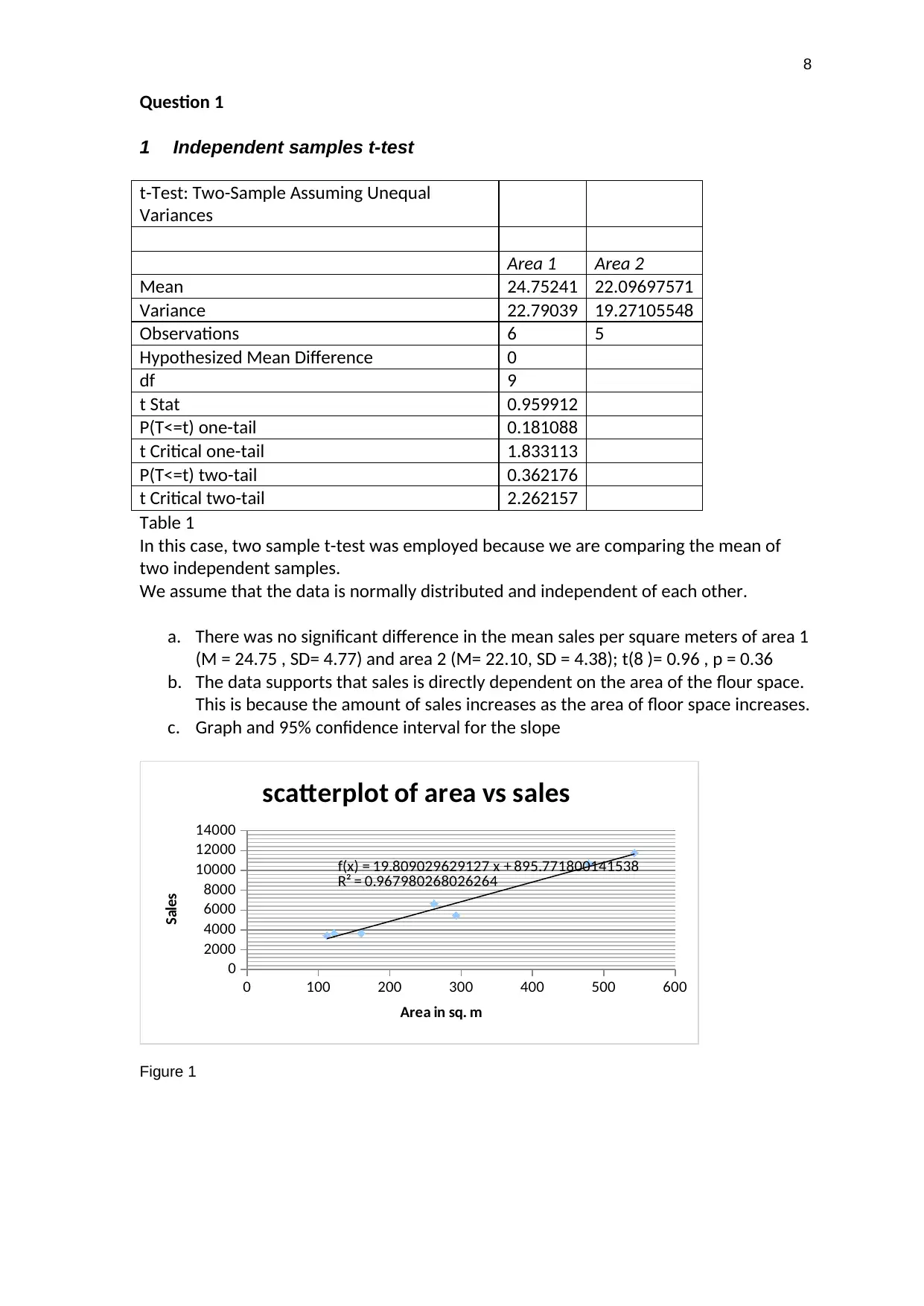
1 Independent samples t-test
t-Test: Two-Sample Assuming Unequal
Variances
Area 1 Area 2
Mean 24.75241 22.09697571
Variance 22.79039 19.27105548
Observations 6 5
Hypothesized Mean Difference 0
df 9
t Stat 0.959912
P(T<=t) one-tail 0.181088
t Critical one-tail 1.833113
P(T<=t) two-tail 0.362176
t Critical two-tail 2.262157
Table 1
In this case, two sample t-test was employed because we are comparing the mean of
two independent samples.
We assume that the data is normally distributed and independent of each other.
a. There was no significant difference in the mean sales per square meters of area 1
(M = 24.75 , SD= 4.77) and area 2 (M= 22.10, SD = 4.38); t(8 )= 0.96 , p = 0.36
b. The data supports that sales is directly dependent on the area of the flour space.
This is because the amount of sales increases as the area of floor space increases.
c. Graph and 95% confidence interval for the slope
0 100 200 300 400 500 600
0
2000
4000
6000
8000
10000
12000
14000
f(x) = 19.809029629127 x + 895.771800141538
R² = 0.967980268026264
scatterplot of area vs sales
Area in sq. m
Sales
Figure 1
Question 1
1 Independent samples t-test
t-Test: Two-Sample Assuming Unequal
Variances
Area 1 Area 2
Mean 24.75241 22.09697571
Variance 22.79039 19.27105548
Observations 6 5
Hypothesized Mean Difference 0
df 9
t Stat 0.959912
P(T<=t) one-tail 0.181088
t Critical one-tail 1.833113
P(T<=t) two-tail 0.362176
t Critical two-tail 2.262157
Table 1
In this case, two sample t-test was employed because we are comparing the mean of
two independent samples.
We assume that the data is normally distributed and independent of each other.
a. There was no significant difference in the mean sales per square meters of area 1
(M = 24.75 , SD= 4.77) and area 2 (M= 22.10, SD = 4.38); t(8 )= 0.96 , p = 0.36
b. The data supports that sales is directly dependent on the area of the flour space.
This is because the amount of sales increases as the area of floor space increases.
c. Graph and 95% confidence interval for the slope
0 100 200 300 400 500 600
0
2000
4000
6000
8000
10000
12000
14000
f(x) = 19.809029629127 x + 895.771800141538
R² = 0.967980268026264
scatterplot of area vs sales
Area in sq. m
Sales
Figure 1
9
Coefficients
std
error t Stat P-value Lower 95% Upper 95%
Intercept
895.77180
0 520.959 1.71946 0.1461 -443.398084
2234.9416
8
sq. m 19.809029 1.61121 12.2944 6.3E-05 15.66726679
23.950792
4
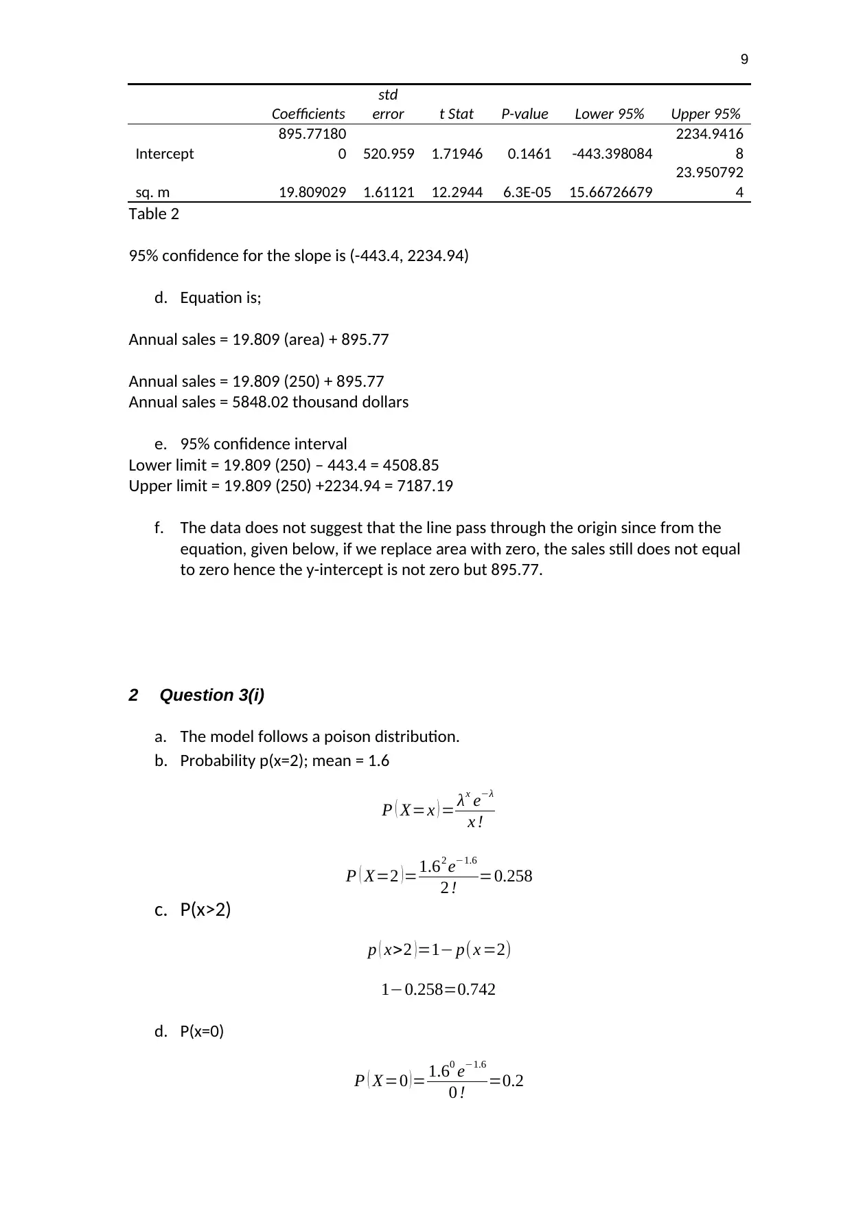
Table 2
95% confidence for the slope is (-443.4, 2234.94)
d. Equation is;
Annual sales = 19.809 (area) + 895.77
Annual sales = 19.809 (250) + 895.77
Annual sales = 5848.02 thousand dollars
e. 95% confidence interval
Lower limit = 19.809 (250) – 443.4 = 4508.85
Upper limit = 19.809 (250) +2234.94 = 7187.19
f. The data does not suggest that the line pass through the origin since from the
equation, given below, if we replace area with zero, the sales still does not equal
to zero hence the y-intercept is not zero but 895.77.
2 Question 3(i)
a. The model follows a poison distribution.
b. Probability p(x=2); mean = 1.6
P ( X=x ) = λx e−λ
x !
P ( X=2 )=1.62 e−1.6
2 ! =0.258
c. P(x>2)
p ( x>2 ) =1− p( x =2)
1−0.258=0.742
d. P(x=0)
P ( X=0 )= 1.60 e−1.6
0 ! =0.2
Coefficients
std
error t Stat P-value Lower 95% Upper 95%
Intercept
895.77180
0 520.959 1.71946 0.1461 -443.398084
2234.9416
8
sq. m 19.809029 1.61121 12.2944 6.3E-05 15.66726679
23.950792
4
Table 2
95% confidence for the slope is (-443.4, 2234.94)
d. Equation is;
Annual sales = 19.809 (area) + 895.77
Annual sales = 19.809 (250) + 895.77
Annual sales = 5848.02 thousand dollars
e. 95% confidence interval
Lower limit = 19.809 (250) – 443.4 = 4508.85
Upper limit = 19.809 (250) +2234.94 = 7187.19
f. The data does not suggest that the line pass through the origin since from the
equation, given below, if we replace area with zero, the sales still does not equal
to zero hence the y-intercept is not zero but 895.77.
2 Question 3(i)
a. The model follows a poison distribution.
b. Probability p(x=2); mean = 1.6
P ( X=x ) = λx e−λ
x !
P ( X=2 )=1.62 e−1.6
2 ! =0.258
c. P(x>2)
p ( x>2 ) =1− p( x =2)
1−0.258=0.742
d. P(x=0)
P ( X=0 )= 1.60 e−1.6
0 ! =0.2
⊘ This is a preview!⊘
Do you want full access?
Subscribe today to unlock all pages.
Trusted by 1+ million students worldwide
10
3 T-test: Two-sample assuming unequal variances
Question 3(ii)
t-Test: Two-Sample Assuming Unequal
Variances
Current
Process
New Process
Mean 75.71428571 67.8333333
3
Variance 36.9047619 24.9666666
7
Observations 7 6
Hypothesized Mean Difference 0
df 11
t Stat 2.565953151
P(T<=t) one-tail 0.013119442
t Critical one-tail 1.795884819
P(T<=t) two-tail 0.026238884
t Critical two-tail 2.20098516
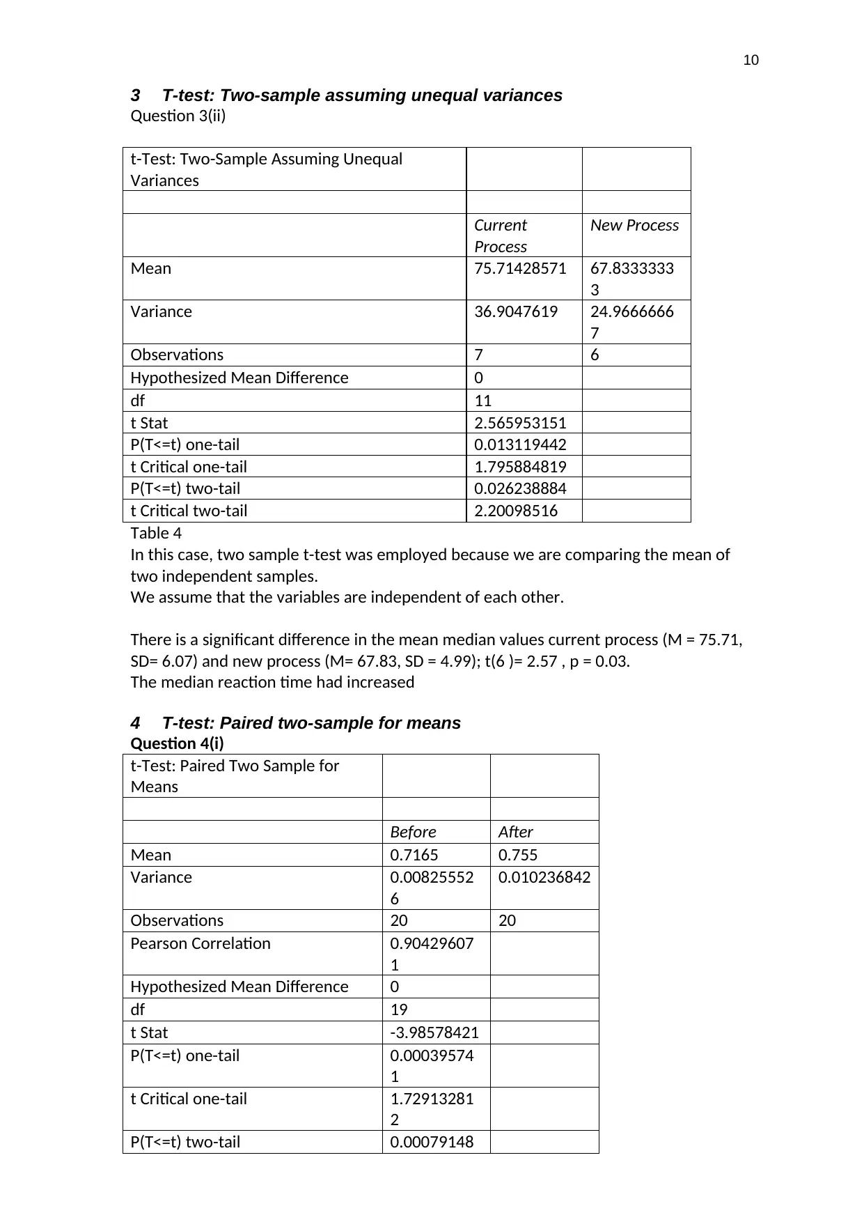
Table 4
In this case, two sample t-test was employed because we are comparing the mean of
two independent samples.
We assume that the variables are independent of each other.
There is a significant difference in the mean median values current process (M = 75.71,
SD= 6.07) and new process (M= 67.83, SD = 4.99); t(6 )= 2.57 , p = 0.03.
The median reaction time had increased
4 T-test: Paired two-sample for means
Question 4(i)
t-Test: Paired Two Sample for
Means
Before After
Mean 0.7165 0.755
Variance 0.00825552
6
0.010236842
Observations 20 20
Pearson Correlation 0.90429607
1
Hypothesized Mean Difference 0
df 19
t Stat -3.98578421
P(T<=t) one-tail 0.00039574
1
t Critical one-tail 1.72913281
2
P(T<=t) two-tail 0.00079148
3 T-test: Two-sample assuming unequal variances
Question 3(ii)
t-Test: Two-Sample Assuming Unequal
Variances
Current
Process
New Process
Mean 75.71428571 67.8333333
3
Variance 36.9047619 24.9666666
7
Observations 7 6
Hypothesized Mean Difference 0
df 11
t Stat 2.565953151
P(T<=t) one-tail 0.013119442
t Critical one-tail 1.795884819
P(T<=t) two-tail 0.026238884
t Critical two-tail 2.20098516
Table 4
In this case, two sample t-test was employed because we are comparing the mean of
two independent samples.
We assume that the variables are independent of each other.
There is a significant difference in the mean median values current process (M = 75.71,
SD= 6.07) and new process (M= 67.83, SD = 4.99); t(6 )= 2.57 , p = 0.03.
The median reaction time had increased
4 T-test: Paired two-sample for means
Question 4(i)
t-Test: Paired Two Sample for
Means
Before After
Mean 0.7165 0.755
Variance 0.00825552
6
0.010236842
Observations 20 20
Pearson Correlation 0.90429607
1
Hypothesized Mean Difference 0
df 19
t Stat -3.98578421
P(T<=t) one-tail 0.00039574
1
t Critical one-tail 1.72913281
2
P(T<=t) two-tail 0.00079148
Paraphrase This Document
Need a fresh take? Get an instant paraphrase of this document with our AI Paraphraser
11
1
t Critical two-tail 2.09302405
4
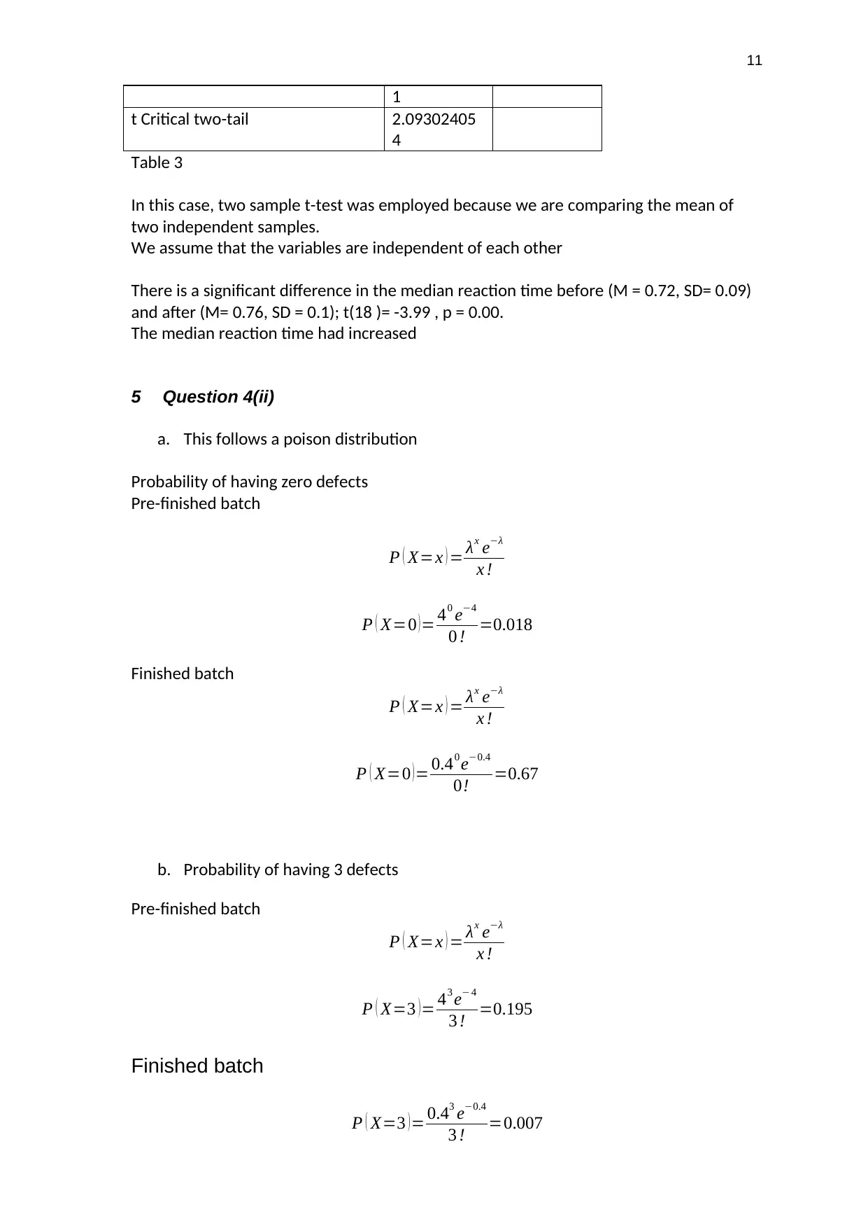
Table 3
In this case, two sample t-test was employed because we are comparing the mean of
two independent samples.
We assume that the variables are independent of each other
There is a significant difference in the median reaction time before (M = 0.72, SD= 0.09)
and after (M= 0.76, SD = 0.1); t(18 )= -3.99 , p = 0.00.
The median reaction time had increased
5 Question 4(ii)
a. This follows a poison distribution
Probability of having zero defects
Pre-finished batch
P ( X=x ) = λx e−λ
x !
P ( X=0 ) = 40 e−4
0 ! =0.018
Finished batch
P ( X=x ) = λx e−λ
x !
P ( X=0 )= 0.40 e−0.4
0! =0.67
b. Probability of having 3 defects
Pre-finished batch
P ( X=x ) = λx e−λ
x !
P ( X=3 )= 43 e− 4
3 ! =0.195
Finished batch
P ( X=3 ) = 0.43 e−0.4
3 ! =0.007
1
t Critical two-tail 2.09302405
4
Table 3
In this case, two sample t-test was employed because we are comparing the mean of
two independent samples.
We assume that the variables are independent of each other
There is a significant difference in the median reaction time before (M = 0.72, SD= 0.09)
and after (M= 0.76, SD = 0.1); t(18 )= -3.99 , p = 0.00.
The median reaction time had increased
5 Question 4(ii)
a. This follows a poison distribution
Probability of having zero defects
Pre-finished batch
P ( X=x ) = λx e−λ
x !
P ( X=0 ) = 40 e−4
0 ! =0.018
Finished batch
P ( X=x ) = λx e−λ
x !
P ( X=0 )= 0.40 e−0.4
0! =0.67
b. Probability of having 3 defects
Pre-finished batch
P ( X=x ) = λx e−λ
x !
P ( X=3 )= 43 e− 4
3 ! =0.195
Finished batch
P ( X=3 ) = 0.43 e−0.4
3 ! =0.007
12
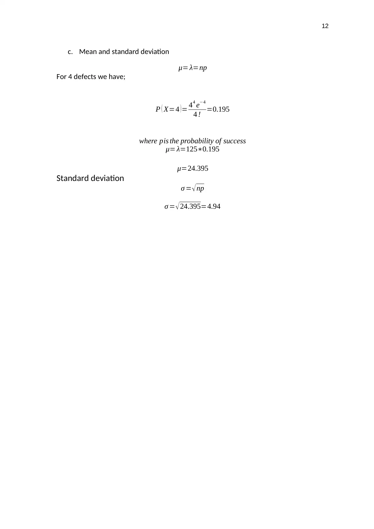
c. Mean and standard deviation
μ= λ=np
For 4 defects we have;
P ( X=4 )= 44 e−4
4 ! =0.195
where pis the probability of success
μ= λ=125∗0.195
μ=24.395
Standard deviation
σ = √ np
σ = √24.395=4.94
c. Mean and standard deviation
μ= λ=np
For 4 defects we have;
P ( X=4 )= 44 e−4
4 ! =0.195
where pis the probability of success
μ= λ=125∗0.195
μ=24.395
Standard deviation
σ = √ np
σ = √24.395=4.94
⊘ This is a preview!⊘
Do you want full access?
Subscribe today to unlock all pages.
Trusted by 1+ million students worldwide
1 out of 12
Your All-in-One AI-Powered Toolkit for Academic Success.
+13062052269
info@desklib.com
Available 24*7 on WhatsApp / Email
![[object Object]](/_next/static/media/star-bottom.7253800d.svg)
Unlock your academic potential
Copyright © 2020–2026 A2Z Services. All Rights Reserved. Developed and managed by ZUCOL.