University Statistics of Management Analysis Report - Module 1

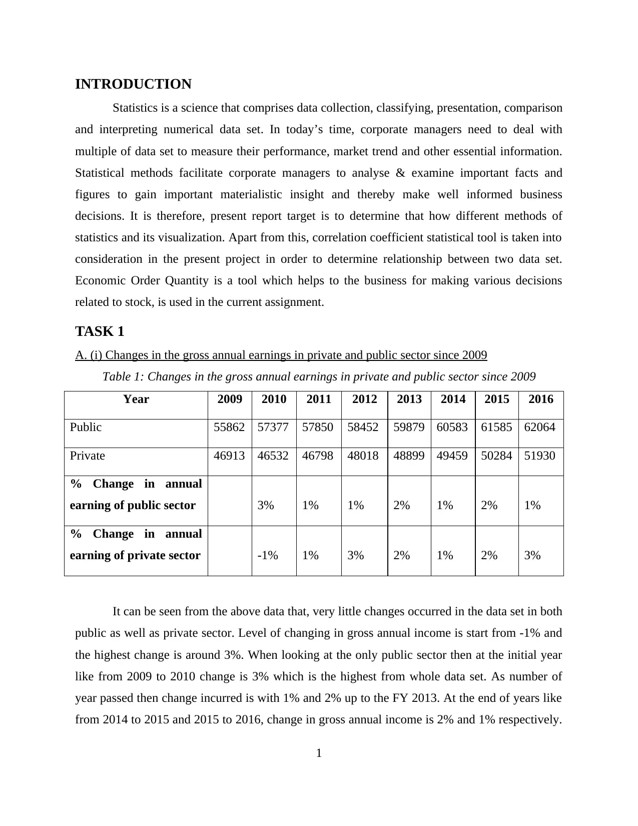
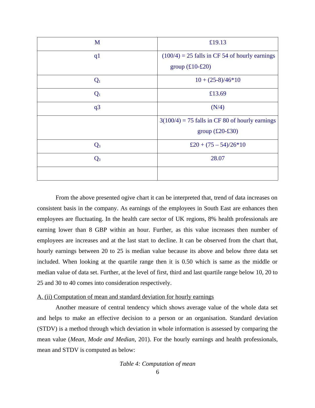
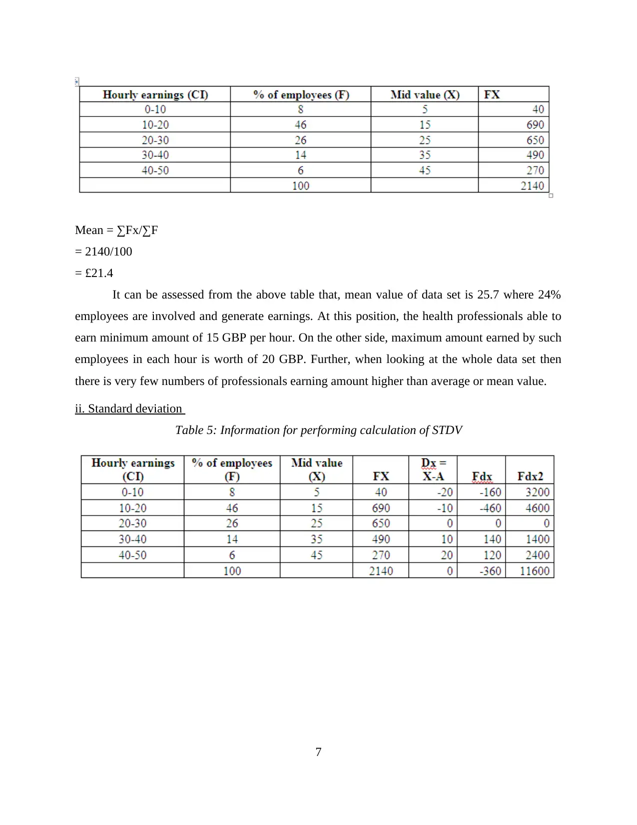
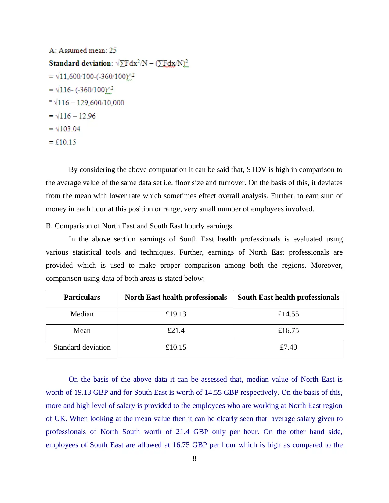
This report provides a comprehensive analysis of statistical data, covering various aspects of management statistics. It begins with an examination of changes in gross annual earnings in the public and private sectors, including the gap between male and female earnings, using tables and illustrations. The report then delves into creating an Ogive graph to estimate median hourly earnings and quartiles, followed by the computation of mean and standard deviation for hourly earnings. A comparison of hourly earnings between the North East and South East regions is also presented. Furthermore, the report explores the relationship between floor area and turnover using scatter diagrams, line of best fit equations, and correlation coefficients. The Economic Order Quantity (EOQ) is calculated, and the impact of changes in EOQ on costs is analyzed. The report concludes with scatter diagrams and line charts illustrating the relationship between size and turnover. The report utilizes various statistical tools and techniques to provide valuable insights into the data.

STATISTICS OF
MANAGEMENT

TABLE OF CONTENTS
INTRODUCTION...........................................................................................................................1
TASK 1............................................................................................................................................1
A. (i) Changes in the gross annual earnings in private and public sector since 2009............1
A. (ii) Gap among male and female gross annual earnings....................................................2
TASK 2............................................................................................................................................4
A. (i) Creating Ogive graph to determine estimate the median hourly earnings & quartiles.4
A. (ii) Computation of mean and standard deviation for hourly earnings..............................6
ii. Standard deviation .............................................................................................................7
B. Comparison of North East and South East hourly earnings..............................................8
A. Scatter diagram and discussion among floor area and turnover........................................9
B. Line of best fit equation...................................................................................................10
C. Calculation of turnover at outlet size of 30 sqm..............................................................10
D. Correlation coefficient.....................................................................................................11
E. Statistical validity.............................................................................................................11
TASK 3..........................................................................................................................................12
B. (a). Calculation of number of deliveries..........................................................................12
B. (b) Calculation of number of bottles sold of olive oil......................................................12
B. (c). Calculation of economic order quantity....................................................................13
B. (d) Finding cost due to changing in EOQ........................................................................14
TASK 4..........................................................................................................................................15
A. Scatter diagram of size versus turnover...........................................................................15
B. Producing line chart.........................................................................................................15
CONCLUSION..............................................................................................................................16
REFERENCES..............................................................................................................................17

INDEX OF TABLES
Table 1: Changes in the gross annual earnings in private and public sector since 2009.................1
Table 2: Gap among male and female gross annual earnings..........................................................2
Table 3: Information for Ogive chart...............................................................................................4
Table 4: Computation of mean........................................................................................................6
Table 5: Information for performing calculation of STDV.............................................................7
Table 6: Computing number of bottles..........................................................................................12
Table 7: Computing EOQ..............................................................................................................13
Table 8: Cost at various EOQ level...............................................................................................14

ILLUSTRATION INDEX
Illustration 1: Male and female earnings from private and public sector........................................3
Illustration 2: Male and female earnings from private and public sector........................................4
Illustration 3: Ogive chart................................................................................................................5
Illustration 4: Line chart on gross annual earnings from private and public sectors.....................15

INTRODUCTION
Statistics is a science that comprises data collection, classifying, presentation, comparison
and interpreting numerical data set. In today’s time, corporate managers need to deal with
multiple of data set to measure their performance, market trend and other essential information.
Statistical methods facilitate corporate managers to analyse & examine important facts and
figures to gain important materialistic insight and thereby make well informed business
decisions. It is therefore, present report target is to determine that how different methods of
statistics and its visualization. Apart from this, correlation coefficient statistical tool is taken into
consideration in the present project in order to determine relationship between two data set.
Economic Order Quantity is a tool which helps to the business for making various decisions
related to stock, is used in the current assignment.
TASK 1
A. (i) Changes in the gross annual earnings in private and public sector since 2009
Table 1: Changes in the gross annual earnings in private and public sector since 2009
Year 2009 2010 2011 2012 2013 2014 2015 2016
Public 55862 57377 57850 58452 59879 60583 61585 62064
Private 46913 46532 46798 48018 48899 49459 50284 51930
% Change in annual
earning of public sector 3% 1% 1% 2% 1% 2% 1%
% Change in annual
earning of private sector -1% 1% 3% 2% 1% 2% 3%
It can be seen from the above data that, very little changes occurred in the data set in both
public as well as private sector. Level of changing in gross annual income is start from -1% and
the highest change is around 3%. When looking at the only public sector then at the initial year
like from 2009 to 2010 change is 3% which is the highest from whole data set. As number of
year passed then change incurred is with 1% and 2% up to the FY 2013. At the end of years like
from 2014 to 2015 and 2015 to 2016, change in gross annual income is 2% and 1% respectively.
1

By considering this trend of change in gross profit, the employees must take corrective actions
for enhancing this particular income level. When visualising to the private sector then change in
earnings are comparatively high. At the initial year i.e. 2009 to 2010 it was in negative like -1%
but after that increase with 3% and 2% at most of the times.
A. (ii) Gap among male and female gross annual earnings
Table 2: Gap among male and female gross annual earnings
Year 2009 2010 2011 2012 2013 2014 2015 2016
Median gross annual
earnings (Male)
Public sector 30638 31264 31380 31816 32541 32878 33685 34011
Private sector 27362 27000 27233 27705 28201 28442 28881 29679
Total 58000 58264 58613 59521 60742 61320 62566 63690
Median gross annual
earnings (Female)
Public sector 25224 26113 26470 26636 27338 27705 27900 28053
Private sector 19551 19532 19565 20313 20698 21017 21403 22251
Total 44775 45645 46035 46949 48036 48722 49303 50304
Change in pay across
gender (Total of male-
Total of female) 13225 12619 12578 12572 12706 12598 13263 13386
2

Illustration 1: Male and female earnings from private and public sector
3

Illustration 2: Male and female earnings from private and public sector
Gap in the gross earnings of employees like male and female on annual basis is with the
high rate which is not better and profitable for them. At the very initial level i.e. in 2009 gap is
worth of 13225 GBP and after that reducing consistently from the whole data set. At the end of
accounting period 2014 gap in male and female incomes is worth of 12598 which is lower as
compared to the initial year. When looking at the last two years then it is 13263 GBP and 13386
GBP in FY 2015 and 2016 respectively. Further, this overall trend of gap in earnings is poor and
create impact on the financial position of workers. In order to manage this position, the
government of country must interfere and take corrective actions where required (Gaile and
Willmott, 2013).
TASK 2
A. (i) Creating Ogive graph to determine estimate the median hourly earnings & quartiles
Table 3: Information for Ogive chart
Hourly Earnings F CF
Below 10 8 8
10 but under 15 22 30
4

15 but under 20 24 54
20 but under 25 14 68
25 but under 30 12 80
30 but under 40 14 94
40 but under 50 6 100
Illustration 3: Ogive chart
Median L1 + (N/2) – c/F*i
L1: lower limit
N: ∑F
c - Cumulative frequency of previous class
interval
i: Class interval
m (N/2) = (100/2) = 50 falls in CF 54 of hourly
earnings group (£10-£20)
L1: 10
N: 100
c - 8
i: 10
M 10 + [(50-8)/46 * 10
5

M £19.13
q1 (100/4) = 25 falls in CF 54 of hourly earnings
group (£10-£20)
Q1 10 + (25-8)/46*10
Q1 £13.69
q3 (N/4)
3(100/4) = 75 falls in CF 80 of hourly earnings
group (£20-£30)
Q3 £20 + (75 – 54)/26*10
Q3 28.07
From the above presented ogive chart it can be interpreted that, trend of data increases on
consistent basis in the company. As earnings of the employees in South East are enhances then
employees are fluctuating. In the health care sector of UK regions, 8% health professionals are
earning lower than 8 GBP within an hour. Further, as this value increases then number of
employees are increases and at the last start to decline. It can be observed from the chart that,
hourly earnings between 20 to 25 is median value because its above and below three data set
included. When looking at the quartile range then it is 0.50 which is same as the middle or
median value of data set. Further, at the level of first, third and last quartile range below 10, 20 to
25 and 30 to 40 comes into consideration respectively.
A. (ii) Computation of mean and standard deviation for hourly earnings
Another measure of central tendency which shows average value of the whole data set
and helps to make an effective decision to a person or an organisation. Standard deviation
(STDV) is a method through which deviation in whole information is assessed by comparing the
mean value (Mean, Mode and Median, 201). For the hourly earnings and health professionals,
mean and STDV is computed as below:
Table 4: Computation of mean
6

Mean = ∑Fx/∑F
= 2140/100
= £21.4
It can be assessed from the above table that, mean value of data set is 25.7 where 24%
employees are involved and generate earnings. At this position, the health professionals able to
earn minimum amount of 15 GBP per hour. On the other side, maximum amount earned by such
employees in each hour is worth of 20 GBP. Further, when looking at the whole data set then
there is very few numbers of professionals earning amount higher than average or mean value.
ii. Standard deviation
Table 5: Information for performing calculation of STDV
7

By considering the above computation it can be said that, STDV is high in comparison to
the average value of the same data set i.e. floor size and turnover. On the basis of this, it deviates
from the mean with lower rate which sometimes effect overall analysis. Further, to earn sum of
money in each hour at this position or range, very small number of employees involved.
B. Comparison of North East and South East hourly earnings
In the above section earnings of South East health professionals is evaluated using
various statistical tools and techniques. Further, earnings of North East professionals are
provided which is used to make proper comparison among both the regions. Moreover,
comparison using data of both areas is stated below:
Particulars North East health professionals South East health professionals
Median £19.13 £14.55
Mean £21.4 £16.75
Standard deviation £10.15 £7.40
On the basis of the above data it can be assessed that, median value of North East is
worth of 19.13 GBP and for South East is worth of 14.55 GBP respectively. On the basis of this,
more and high level of salary is provided to the employees who are working at North East region
of UK. When looking at the mean value then it can be clearly seen that, average salary given to
professionals of North South worth of 21.4 GBP only per hour. On the other hand side,
employees of South East are allowed at 16.75 GBP per hour which is high as compared to the
8