Project: Advanced Thermal and Fluid Engineering Analysis

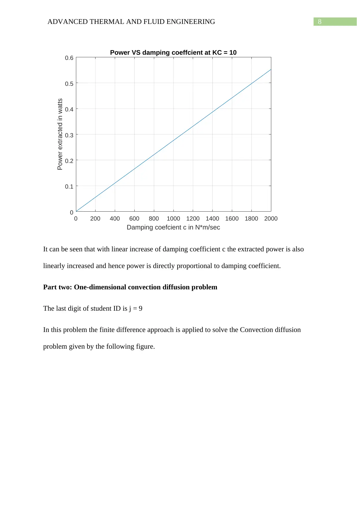
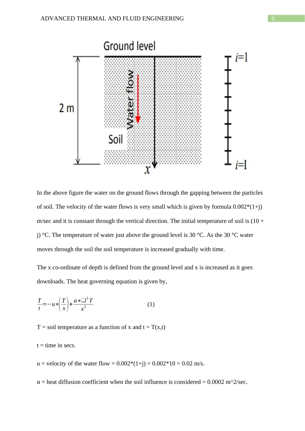
This project report presents a comprehensive analysis of advanced thermal and fluid engineering principles, encompassing two distinct parts. The first part focuses on a simple initial value problem, specifically the vibration of a cylinder subjected to oscillatory flow. The student derives the equation of motion and develops a numerical method, employing the Finite Difference Method (FDM), to predict the cylinder's vibration. MATLAB code is provided to simulate the cylinder's behavior and calculate the power extracted from an electricity generator, demonstrating the relationship between the KC number and power output, as well as the effect of damping coefficient. The second part addresses a one-dimensional convection-diffusion problem, where the FDM is used to solve the heat transfer equation in soil. The student models the temperature distribution within the soil as water flows through it, with MATLAB code used to plot temperature variations over time and depth. The project investigates the impact of the heat diffusion coefficient on the temperature profile, demonstrating how changes in this parameter affect the time required for a specific temperature to be reached at a certain depth.

Running head: ADVANCED THERMAL AND FLUID ENGINEERING
ADVANCED THERMAL AND FLUID ENGINEERING
Name of the Student
Name of the University
Author Note

1ADVANCED THERMAL AND FLUID ENGINEERING
Part one: Simple initial value problem
j = 9
Given,
Um= 1 + 9/10 = 1.9 m/s
U0 = 0.1*1.9 = 0.19 m/s
D = 10 + 9 = 19 cm = 19*10^(-2) m
Mass of cylinder m = 50 kgs
Water density ρ = 1024 kg/m^3
Stiffness of spring K = 200 N/m
Damping coefficient c = 10 N*m/sec
md = 1 and CA = CD = 1.
The KC number is given by,
KC = Um*T/D
Hence, for KC = 2 => T = 2*D/Um = 0.2 sec.
Time period is divided in small time intervals.
Flow velocity V r =u−V
Now, initially, V r (0) = V(0) = U0 and V r (end) = U0
Now, the Morrison equation is given by,
Fwater=C A∗md∗( d V r
dt )+ ( ½ )∗ρ∗CD∗A P∗|V r |∗V r

2ADVANCED THERMAL AND FLUID ENGINEERING
Now, Fwater = m*g = 1024*(2*pi*D/2)*L*9.8 = 5990 N.
Now, this force will balance the hydrodynamic force and hence will cancel out
Hence, in finite difference method the Morrison equation will be given by,
CA∗md∗Vr ( t +1 )−Vr ( t )
dt + ( ½ )∗ρ∗CD∗AP∗|V r ( t )|∗V r ( t )=0
 Vr ( t +1 )= (− ( ½ )∗ρ∗C D∗AP∗|V r ( t )|∗V r ( t ) ) dt /(C A∗md )+ Vr ( t )
Now, after obtaining V r (t), V(t) can be found for entire time period of T.
Then the power P can be calculated by numerical integration with the formula
P = 1
N ∑
n=1
N
c∗(V ¿¿ n)2 ¿
Where, N = the number of points T is divided.
MATLAB code for Vibration speed:
function P = question1(KC)
j = 9;
Um = 1 + (j/10); % amplitude of oscillatory flow in m/s
U0 = 0.1*Um; % steady state flow in m/s
D = (10 + j)*1e-2; % diameter in m
L = 1;
m = 50;
rho = 1024;
K = 200;

3ADVANCED THERMAL AND FLUID ENGINEERING
c = 10;
Ap = 2*pi*(D/2)*L; % projected area is the surface area of the cylinder
md = 1; % added mass coefficient
CA = 1.8; CD = 1.8; T = KC*D/Um;
Fwater = 1024*(2*pi*D/2)*L*9.8;
t = linspace(0,T,150);
dt = t(2)- t(1);
Vr = U0 + Um.*sin(2*pi*t/T);
Vr(1) = U0; Vr(end) = U0;
%%% solving Vr(t) by FDM
for idt = 2:length(t)-2
Vr(idt+1) = (- (1/2)*rho*CD*Ap*abs(Vr(idt))*Vr(idt))*dt/(CA*md) + Vr(idt);
end
V = Vr;
plot(t,V,'b-')
xlabel('Time t in secs')
ylabel('Vibration speed in m/sec')
title('Vibration speed with respect to time')

4ADVANCED THERMAL AND FLUID ENGINEERING
grid on
%%% computing Power extracted P from electricity generator
P=0;
for i=1:length(t)
P = P + c*(abs(V(i))^i)^2;
end
P = P/length(t);
fprintf('The total power P extracted from generator for KC number =2 is %.3f Watts',P)
end
Output:

5ADVANCED THERMAL AND FLUID ENGINEERING
0 0.02 0.04 0.06 0.08 0.1 0.12 0.14 0.16 0.18 0.2
Time t in secs
0
0.05
0.1
0.15
0.2
0.25
0.3
Vibration speed in m/sec
Vibration speed with respect to time
The total power P extracted from generator for KC number =2 is 0.003 Watts
P =
0.0028
Now, for finding the relationship between KC number and power the MATLAB code is
modified and code for graph generation is given below.
MATLAB code:
KC = 2:2:20; % variation of KC number
c= 100;
for i=1:length(KC)
P(i) = question1(KC(i),c);

6ADVANCED THERMAL AND FLUID ENGINEERING
end
plot(KC,P)
xlabel('KC number')
ylabel('Power extracted in watts')
grid on
title('Power VS KC at c = 100 N*m/sec')
Plot:
2 4 6 8 10 12 14 16 18 20
KC number
0.0276
0.02765
0.0277
0.02775
Power extracted in watts
Power VS KC at c = 100 N*m/sec
It can be seen from the above graph that as the KC number is increased the power extracted
has been decreased this is because KC number is inversely proportional to the power.
Now, KC number is kept constant at 10 and value of c is varied in the range 0 to 2000
N*m/sec by step of 50.

7ADVANCED THERMAL AND FLUID ENGINEERING
MATLAB code:
KC = 10;
c = 0:50:2000;
for i=1:length(c)
P(i) = question1(KC,c(i));
end
plot(c,P)
xlabel('Damping coefcient c in N*m/sec')
ylabel('Power extracted in watts')
grid on
title('Power VS damping coeffcient at KC = 10')
Output:

8ADVANCED THERMAL AND FLUID ENGINEERING
0 200 400 600 800 1000 1200 1400 1600 1800 2000
Damping coefcient c in N*m/sec
0
0.1
0.2
0.3
0.4
0.5
0.6
Power extracted in watts
Power VS damping coeffcient at KC = 10
It can be seen that with linear increase of damping coefficient c the extracted power is also
linearly increased and hence power is directly proportional to damping coefficient.
Part two: One-dimensional convection diffusion problem
The last digit of student ID is j = 9
In this problem the finite difference approach is applied to solve the Convection diffusion
problem given by the following figure.

9ADVANCED THERMAL AND FLUID ENGINEERING
In the above figure the water on the ground flows through the gapping between the particles
of soil. The velocity of the water flows is very small which is given by formula 0.002*(1+j)
m/sec and it is constant through the vertical direction. The initial temperature of soil is (10 +
j) °C. The temperature of water just above the ground level is 30 °C. As the 30 °C water
moves through the soil the soil temperature is increased gradually with time.
The x co-ordinate of depth is defined from the ground level and x is increased as it goes
downloads. The heat governing equation is given by,
T
t =−u∗( T
x )+ α∗❑2 T
x2 (1)
T = soil temperature as a function of x and t = T(x,t)
t = time in secs.
u = velocity of the water flow = 0.002*(1+j) = 0.002*10 = 0.02 m/s.
α = heat diffusion coefficient when the soil influence is considered = 0.0002 m^2/sec.

10ADVANCED THERMAL AND FLUID ENGINEERING
The depth of soil from x=0 to x=2 meters is divided into 200 cells.
Hence, x= 0 is the first cell and x= 2 is the 200th cell.
Hence, by finite difference approximation the differential equation (1) becomes
T ( x , t +dt ) – T ( x , t )
dt =−u∗T ( x +dx , t ) – T ( x , t )
dx + α∗T ( x +dx ,t ) – 2∗T ( x , t ) +T ( x−dx , t )
d x2
OR,
T ( x , t+dt )= (−u∗T ( x+ dx , t ) – T ( x , t )
dx + α∗T ( x +dx , t ) – 2∗T ( x ,t ) +T ( x−dx , t )
d x2 )∗dt+T (x , t )
Where, i-1 to i+1 varies from temperature at 1st to 200th cell or point.
Boundary conditions are T|x=0 = 30 °C, T
x =0 at x= 2.
Also, T(i) = (10 + j) = (10+9) °C = 19 °C initially for all i.
T
x =0 at x= 2 => (T(200,t) – T(199,t))/dx = 0
Hence, T(200,t) = T(199,t) Or, T(200,t) = T(199,t)
Hence, by finite difference method temperatures from T(1) to T(199) is calculated and then
the value of T(199) is made equal to T(200).
MATLAB code for temperature plot and T1.5 at α = 0.0002 m^2/sec:
function time25deg = question2(alpha) % heat diffusion coeffcient
u = 0.02; % flow velocity
x= linspace(0,2,200); % dividing 2 meters in 200 cells
dx = x(2) - x(1); % Deep length x increment per step

11ADVANCED THERMAL AND FLUID ENGINEERING
dt = dx; % time t increment per step
t = 0:dt:100; % 0 to 10 secs
T = repmat(19,length(x),length(t)); % initially all T are at 19 degree C
T(1,:) = 30; T(199,:) = T(200,:); % boundary conditions
for idt = 1:length(t)-1
for idx = 2:length(x)-1
T(idx,idt+1) = dt*(-u*(T(idx+1,idt) - T(idx,idt))/dx + alpha*(T(idx+1,idt) - 2*T(idx,idt)
+ T(idx-1,idt))/dx^2) + T(idx,idt); % FDM iteration equation
end
end
T(200,:) = T(199,:);
[xx,tt] = meshgrid(x,t);
mesh(xx,tt,T')
xlabel('Depth in [0,2] m')
ylabel('Time in Sec')
zlabel('Temperature in Degree C')
title('Temperature plot T(x,t)')
grid on