Performance Analysis of 5G New Radio Channel Codes for URLLC Scenarios
VerifiedAdded on 2023/04/24
|15
|3582
|303
Report
AI Summary
This report presents an analysis of channel coding schemes for 5G Ultra-Reliable Low Latency Communication (URLLC) use cases. The study focuses on the performance evaluation of polar codes, LDPC codes, and other channel codes under various parameters relevant to URLLC scenarios. The report includes simulations and comparisons of these codes based on bit error rate (BER), frame error rate (FER), and complexity. The analysis examines the impact of different code lengths (N) and code rates (R) on the performance of the codes. The results demonstrate the performance of the codes under different velocities. Additionally, the report compares the complexity of the URLLC code with existing codes like TBCC, LTE Turbo, and LDPC. The conclusion highlights the suitability of URLLC codes for high-speed train channels, emphasizing their low complexity, high speed capabilities, and low latency. Recommendations for network architecture and communication protocols are also provided.
5G New Radio Channel Codes:
URLLC
Table of Contents
Introduction …………………………………………………………….….…………….2
Coding of HST Channel……………………………………………………….….……...2
Analysis of URLLC at various values of N…………………………………………...….7
Analysis of new channel with various performance rates………………………...……...9
Analysis of URLLC channel with turbo codes,
polar codes, LDPC codes and TBCC codes……………………………………….......11
Analysis of the new channel in various velocities………………………………………13
Complexity performance of URLLC code with existing codes…………………………14
Conclusion……………………………………………………………………………....15
1
Paraphrase This Document
Need a fresh take? Get an instant paraphrase of this document with our AI Paraphraser
ABSTRACT
Channel coding for 5G New Radio is facing modern challenges in upholding and encouraging
various emerging use cases and new applications. Highly developed channel codes for existing
mobile generations are having performance problems for lots of 5G applications. Polar code is
prominent advancement in the channel coding area of this decade. The unprecedented
performance of polar codes compelled 3GPP to adopt them for 5G eMBB control channels and
over the physical broadcast channel.
This paper focuses on channel coding schemes particularly for 5G-URLLC use case and
evaluating the performance of polar codes for this scenario. Polar, LDPC codes and other
channel codes are compared using various parameters desired for URLLC scenario.
INTRODUCTION
It is also known as the short- length codes of Ultra-Reliable Latency Communication. It has high
reliability and low latency and error rate is low than 10-9. For high reliability URLLC channel code is use
at low error rate. Information block size should be less than 1000 bits find that existing code like LDPC,
TB-CC, Polar has large block size and give big differences with small block size also satisfying by
URLLC code. Because of low rate and low complexity. The 5G-URLLC channel has strict
requirement on the ultrahigh reliability and ultralow latency. The low decoding complexity and
latency with high reliability certainly makes polar code a strong contender in this race as well.
METHODS
Coding of HST Channel (URLLC)
The fading characteristics function, y = sqrt (d^-v) * randn (N, 1) and N = 128
clc
clear all
close all
N=128; K=64; Ec=1; N0=2;
initPC(N,K,Ec,N0);
u= (rand(K,1)>0.7)
length(u)
x= pencode(u)
2
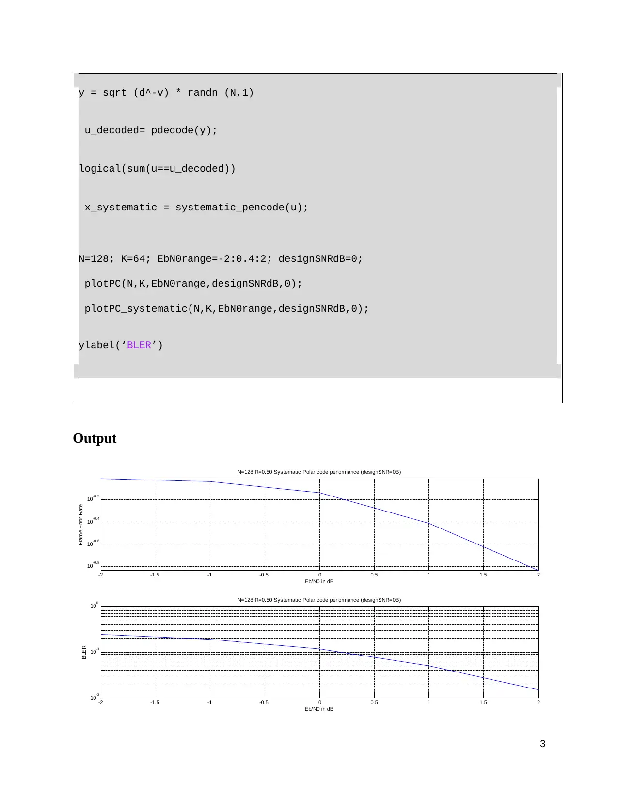
y = sqrt (d^-v) * randn (N,1)
u_decoded= pdecode(y);
logical(sum(u==u_decoded))
x_systematic = systematic_pencode(u);
N=128; K=64; EbN0range=-2:0.4:2; designSNRdB=0;
plotPC(N,K,EbN0range,designSNRdB,0);
plotPC_systematic(N,K,EbN0range,designSNRdB,0);
ylabel(‘BLER’)
Output
-2 -1.5 -1 -0.5 0 0.5 1 1.5 2
10-0.8
10-0.6
10-0.4
10-0.2
N=128 R=0.50 Systematic Polar code performance (designSNR=0B)
Eb/N0 in dB
Frame Error Rate
-2 -1.5 -1 -0.5 0 0.5 1 1.5 2
10-2
10-1
100 N=128 R=0.50 Systematic Polar code performance (designSNR=0B)
Eb/N0 in dB
BLER
3
⊘ This is a preview!⊘
Do you want full access?
Subscribe today to unlock all pages.
Trusted by 1+ million students worldwide
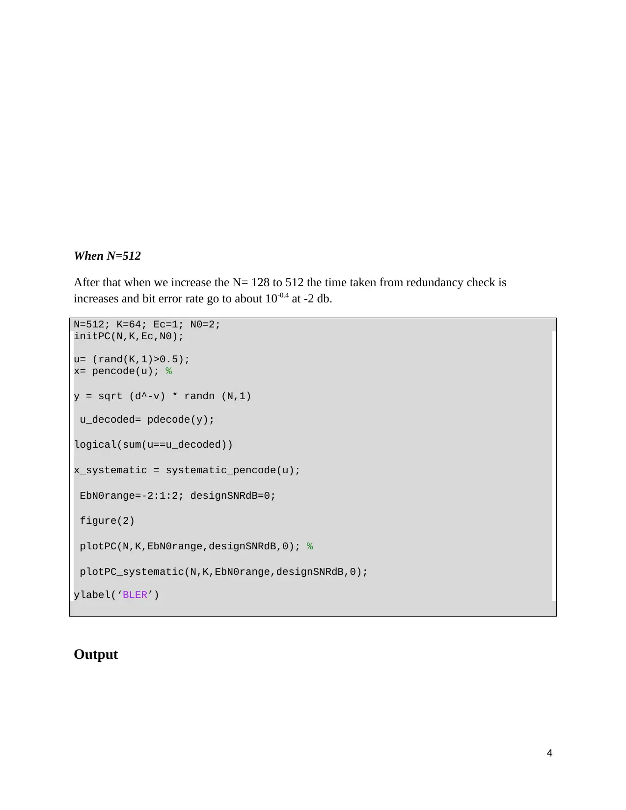
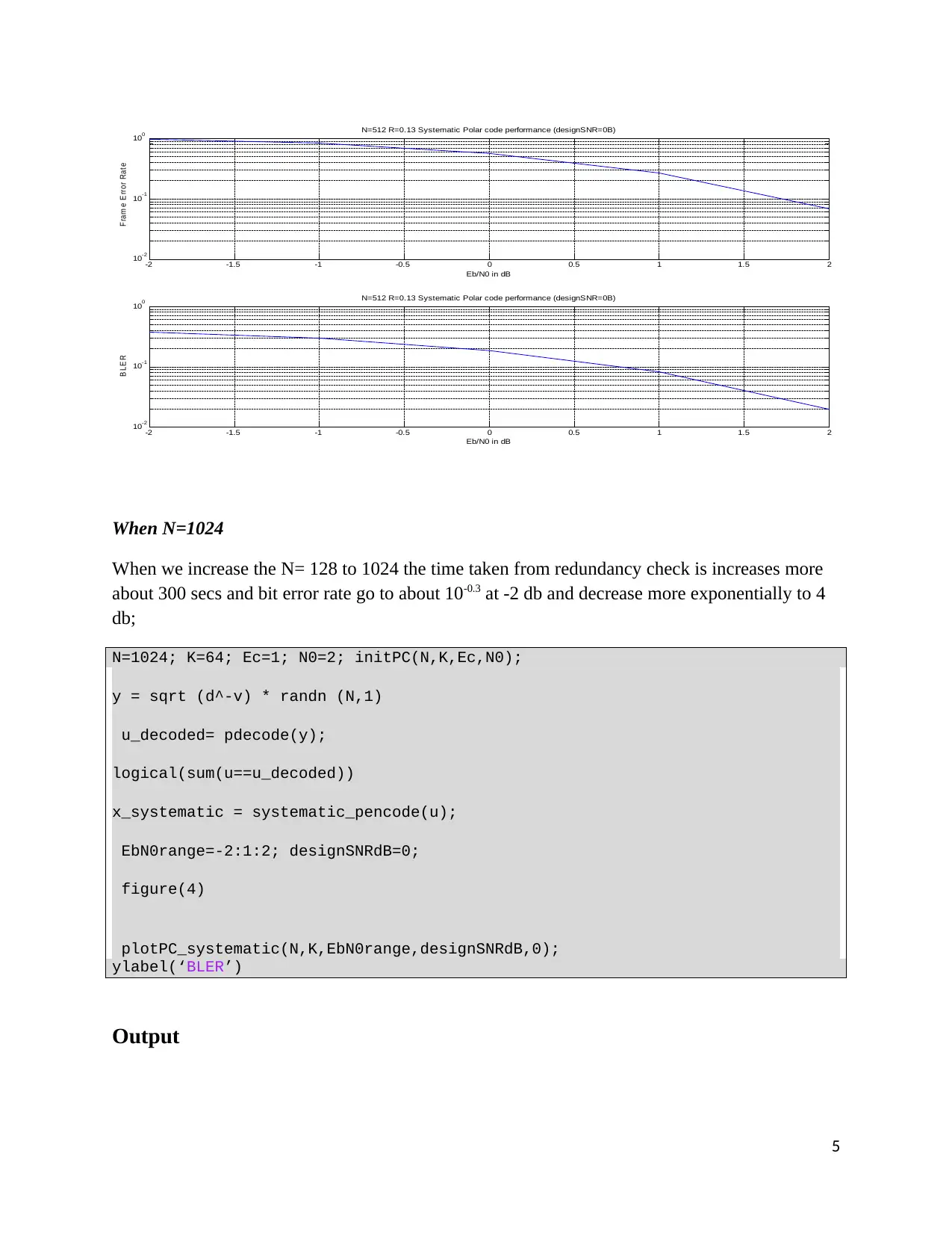
When N=512
After that when we increase the N= 128 to 512 the time taken from redundancy check is
increases and bit error rate go to about 10-0.4 at -2 db.
N=512; K=64; Ec=1; N0=2;
initPC(N,K,Ec,N0);
u= (rand(K,1)>0.5);
x= pencode(u); %
y = sqrt (d^-v) * randn (N,1)
u_decoded= pdecode(y);
logical(sum(u==u_decoded))
x_systematic = systematic_pencode(u);
EbN0range=-2:1:2; designSNRdB=0;
figure(2)
plotPC(N,K,EbN0range,designSNRdB,0); %
plotPC_systematic(N,K,EbN0range,designSNRdB,0);
ylabel(‘BLER’)
Output
4
Paraphrase This Document
Need a fresh take? Get an instant paraphrase of this document with our AI Paraphraser
-2 -1.5 -1 -0.5 0 0.5 1 1.5 2
10
-2
10
-1
10
0 N=512 R=0.13 Systematic Polar code performance (designSNR=0B)
Eb/N0 in dB
F ram e E rror Rate
-2 -1.5 -1 -0.5 0 0.5 1 1.5 2
10
-2
10
-1
10
0 N=512 R=0.13 Systematic Polar code performance (designSNR=0B)
Eb/N0 in dB
B LE R
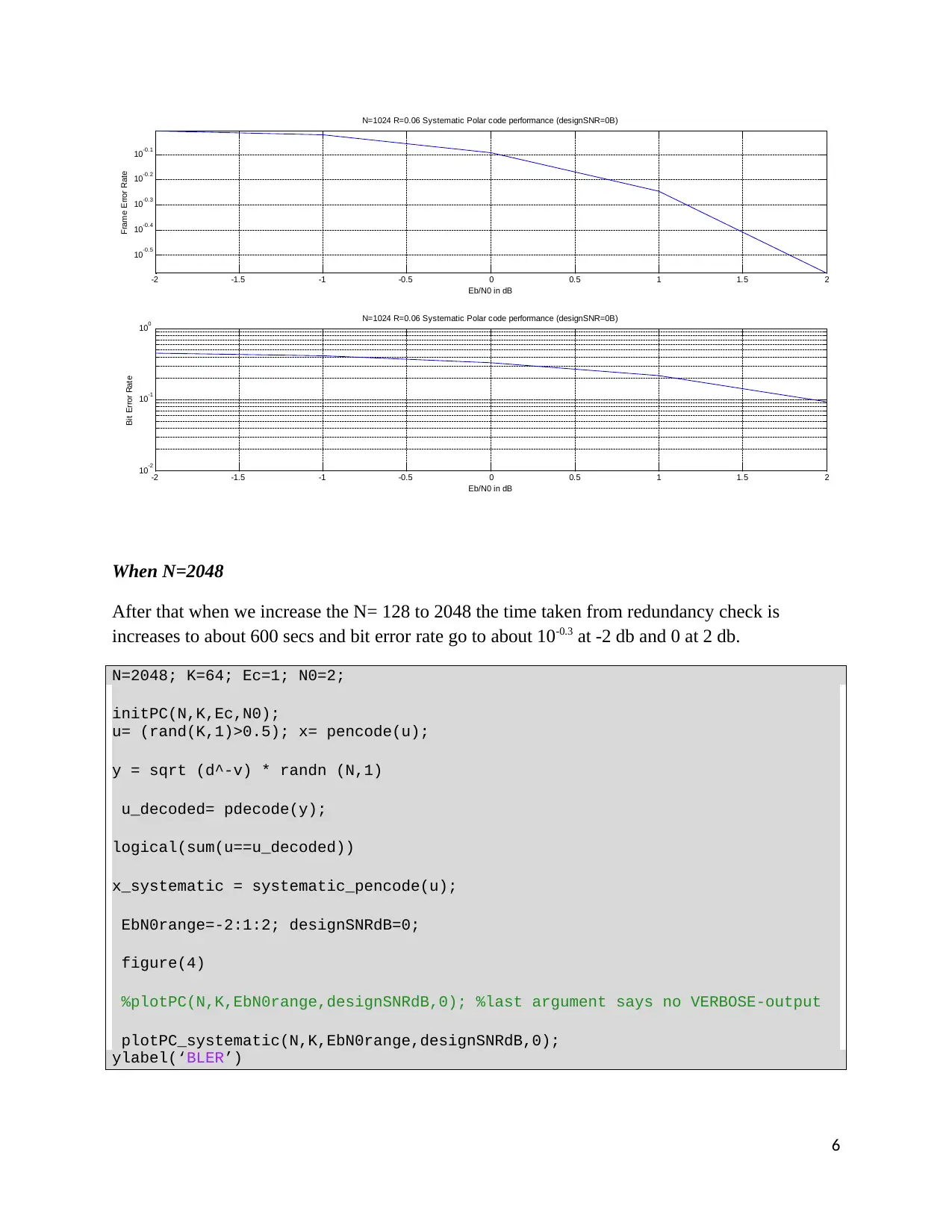
When N=1024
When we increase the N= 128 to 1024 the time taken from redundancy check is increases more
about 300 secs and bit error rate go to about 10-0.3 at -2 db and decrease more exponentially to 4
db;
N=1024; K=64; Ec=1; N0=2; initPC(N,K,Ec,N0);
y = sqrt (d^-v) * randn (N,1)
u_decoded= pdecode(y);
logical(sum(u==u_decoded))
x_systematic = systematic_pencode(u);
EbN0range=-2:1:2; designSNRdB=0;
figure(4)
plotPC_systematic(N,K,EbN0range,designSNRdB,0);
ylabel(‘BLER’)
Output
5
10
-2
10
-1
10
0 N=512 R=0.13 Systematic Polar code performance (designSNR=0B)
Eb/N0 in dB
F ram e E rror Rate
-2 -1.5 -1 -0.5 0 0.5 1 1.5 2
10
-2
10
-1
10
0 N=512 R=0.13 Systematic Polar code performance (designSNR=0B)
Eb/N0 in dB
B LE R
When N=1024
When we increase the N= 128 to 1024 the time taken from redundancy check is increases more
about 300 secs and bit error rate go to about 10-0.3 at -2 db and decrease more exponentially to 4
db;
N=1024; K=64; Ec=1; N0=2; initPC(N,K,Ec,N0);
y = sqrt (d^-v) * randn (N,1)
u_decoded= pdecode(y);
logical(sum(u==u_decoded))
x_systematic = systematic_pencode(u);
EbN0range=-2:1:2; designSNRdB=0;
figure(4)
plotPC_systematic(N,K,EbN0range,designSNRdB,0);
ylabel(‘BLER’)
Output
5
-2 -1.5 -1 -0.5 0 0.5 1 1.5 2
10 -0.5
10 -0.4
10 -0.3
10 -0.2
10 -0.1
N=1024 R=0.06 Systematic Polar code performance (designSNR=0B)
Eb/N0 in dB
Frame Error Rate
-2 -1.5 -1 -0.5 0 0.5 1 1.5 2
10
-2
10
-1
10
0 N=1024 R=0.06 Systematic Polar code performance (designSNR=0B)
Eb/N0 in dB
Bit Error Rate
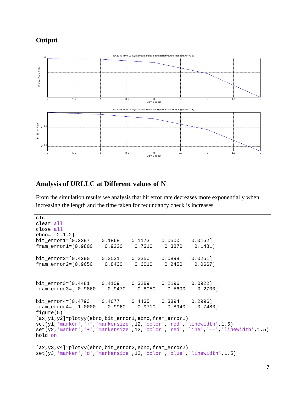
When N=2048
After that when we increase the N= 128 to 2048 the time taken from redundancy check is
increases to about 600 secs and bit error rate go to about 10-0.3 at -2 db and 0 at 2 db.
N=2048; K=64; Ec=1; N0=2;
initPC(N,K,Ec,N0);
u= (rand(K,1)>0.5); x= pencode(u);
y = sqrt (d^-v) * randn (N,1)
u_decoded= pdecode(y);
logical(sum(u==u_decoded))
x_systematic = systematic_pencode(u);
EbN0range=-2:1:2; designSNRdB=0;
figure(4)
%plotPC(N,K,EbN0range,designSNRdB,0); %last argument says no VERBOSE-output
plotPC_systematic(N,K,EbN0range,designSNRdB,0);
ylabel(‘BLER’)
6
10 -0.5
10 -0.4
10 -0.3
10 -0.2
10 -0.1
N=1024 R=0.06 Systematic Polar code performance (designSNR=0B)
Eb/N0 in dB
Frame Error Rate
-2 -1.5 -1 -0.5 0 0.5 1 1.5 2
10
-2
10
-1
10
0 N=1024 R=0.06 Systematic Polar code performance (designSNR=0B)
Eb/N0 in dB
Bit Error Rate
When N=2048
After that when we increase the N= 128 to 2048 the time taken from redundancy check is
increases to about 600 secs and bit error rate go to about 10-0.3 at -2 db and 0 at 2 db.
N=2048; K=64; Ec=1; N0=2;
initPC(N,K,Ec,N0);
u= (rand(K,1)>0.5); x= pencode(u);
y = sqrt (d^-v) * randn (N,1)
u_decoded= pdecode(y);
logical(sum(u==u_decoded))
x_systematic = systematic_pencode(u);
EbN0range=-2:1:2; designSNRdB=0;
figure(4)
%plotPC(N,K,EbN0range,designSNRdB,0); %last argument says no VERBOSE-output
plotPC_systematic(N,K,EbN0range,designSNRdB,0);
ylabel(‘BLER’)
6
⊘ This is a preview!⊘
Do you want full access?
Subscribe today to unlock all pages.
Trusted by 1+ million students worldwide
Output
-2 -1.5 -1 -0.5 0 0.5 1 1.5 2
10
0 N=2048 R=0.03 Systematic Polar code performance (designSNR=0B)
Eb/N0 in dB
Fram e E rror Rate
-2 -1.5 -1 -0.5 0 0.5 1 1.5 2
10 -0.5
10 -0.4
N=2048 R=0.03 Systematic Polar code performance (designSNR=0B)
Eb/N0 in dB
B it E rror Rate
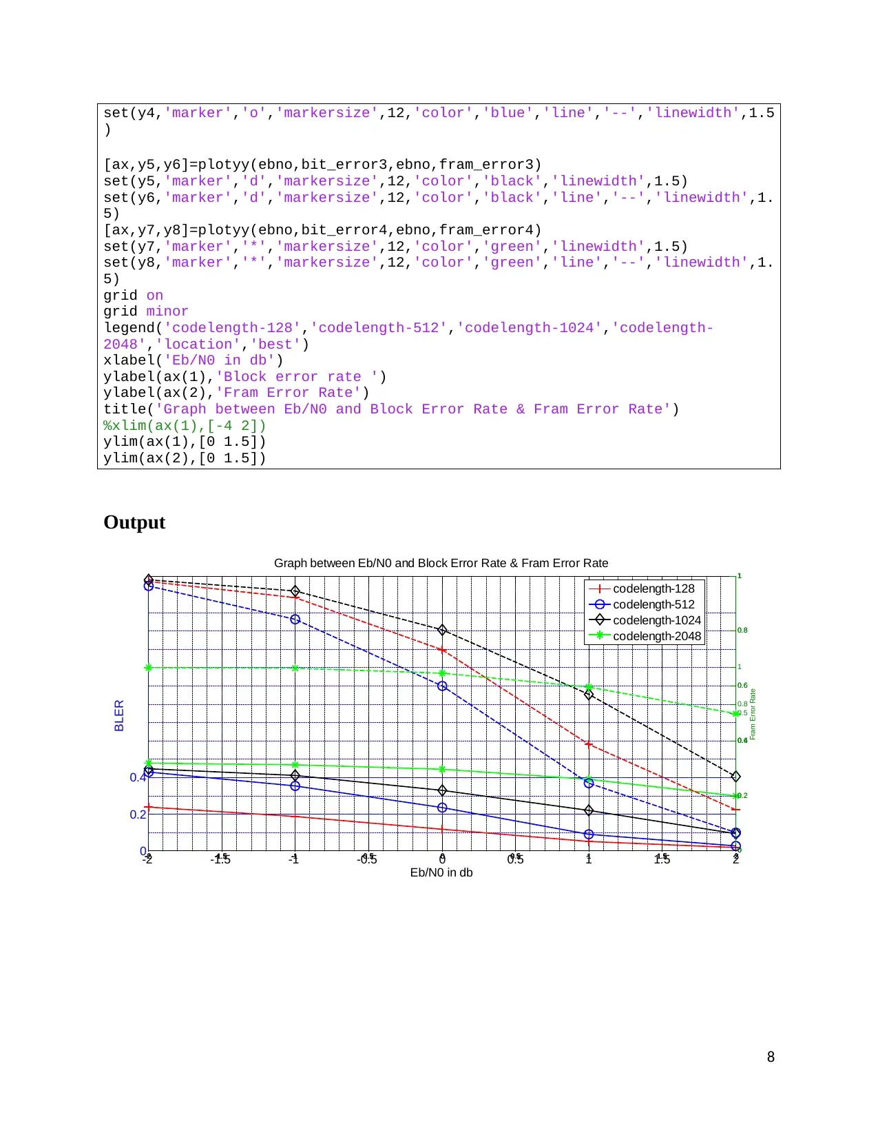
Analysis of URLLC at Different values of N
From the simulation results we analysis that bit error rate decreases more exponentially when
increasing the length and the time taken for redundancy check is increases.
clc
clear all
close all
ebno=[-2:1:2]
bit_error1=[0.2397 0.1868 0.1173 0.0500 0.0152]
fram_error1=[0.9800 0.9220 0.7310 0.3870 0.1481]
bit_error2=[0.4290 0.3531 0.2350 0.0898 0.0251]
fram_error2=[0.9650 0.8430 0.6010 0.2450 0.0667]
bit_error3=[0.4481 0.4109 0.3289 0.2196 0.0922]
fram_error3=[ 0.9860 0.9470 0.8050 0.5690 0.2700]
bit_error4=[0.4793 0.4677 0.4435 0.3894 0.2996]
fram_error4=[ 1.0000 0.9960 0.9710 0.8940 0.7480]
figure(5)
[ax,y1,y2]=plotyy(ebno,bit_error1,ebno,fram_error1)
set(y1,'marker','+','markersize',12,'color','red','linewidth',1.5)
set(y2,'marker','+','markersize',12,'color','red','line','--','linewidth',1.5)
hold on
[ax,y3,y4]=plotyy(ebno,bit_error2,ebno,fram_error2)
set(y3,'marker','o','markersize',12,'color','blue','linewidth',1.5)
7
-2 -1.5 -1 -0.5 0 0.5 1 1.5 2
10
0 N=2048 R=0.03 Systematic Polar code performance (designSNR=0B)
Eb/N0 in dB
Fram e E rror Rate
-2 -1.5 -1 -0.5 0 0.5 1 1.5 2
10 -0.5
10 -0.4
N=2048 R=0.03 Systematic Polar code performance (designSNR=0B)
Eb/N0 in dB
B it E rror Rate
Analysis of URLLC at Different values of N
From the simulation results we analysis that bit error rate decreases more exponentially when
increasing the length and the time taken for redundancy check is increases.
clc
clear all
close all
ebno=[-2:1:2]
bit_error1=[0.2397 0.1868 0.1173 0.0500 0.0152]
fram_error1=[0.9800 0.9220 0.7310 0.3870 0.1481]
bit_error2=[0.4290 0.3531 0.2350 0.0898 0.0251]
fram_error2=[0.9650 0.8430 0.6010 0.2450 0.0667]
bit_error3=[0.4481 0.4109 0.3289 0.2196 0.0922]
fram_error3=[ 0.9860 0.9470 0.8050 0.5690 0.2700]
bit_error4=[0.4793 0.4677 0.4435 0.3894 0.2996]
fram_error4=[ 1.0000 0.9960 0.9710 0.8940 0.7480]
figure(5)
[ax,y1,y2]=plotyy(ebno,bit_error1,ebno,fram_error1)
set(y1,'marker','+','markersize',12,'color','red','linewidth',1.5)
set(y2,'marker','+','markersize',12,'color','red','line','--','linewidth',1.5)
hold on
[ax,y3,y4]=plotyy(ebno,bit_error2,ebno,fram_error2)
set(y3,'marker','o','markersize',12,'color','blue','linewidth',1.5)
7
Paraphrase This Document
Need a fresh take? Get an instant paraphrase of this document with our AI Paraphraser
set(y4,'marker','o','markersize',12,'color','blue','line','--','linewidth',1.5
)
[ax,y5,y6]=plotyy(ebno,bit_error3,ebno,fram_error3)
set(y5,'marker','d','markersize',12,'color','black','linewidth',1.5)
set(y6,'marker','d','markersize',12,'color','black','line','--','linewidth',1.
5)
[ax,y7,y8]=plotyy(ebno,bit_error4,ebno,fram_error4)
set(y7,'marker','*','markersize',12,'color','green','linewidth',1.5)
set(y8,'marker','*','markersize',12,'color','green','line','--','linewidth',1.
5)
grid on
grid minor
legend('codelength-128','codelength-512','codelength-1024','codelength-
2048','location','best')
xlabel('Eb/N0 in db')
ylabel(ax(1),'Block error rate ')
ylabel(ax(2),'Fram Error Rate')
title('Graph between Eb/N0 and Block Error Rate & Fram Error Rate')
%xlim(ax(1),[-4 2])
ylim(ax(1),[0 1.5])
ylim(ax(2),[0 1.5])
Output
-2 -1.5 -1 -0.5 0 0.5 1 1.5 2
0
0.2
0.4
Eb/N0 in db
BLER
Graph between Eb/N0 and Block Error Rate & Fram Error Rate
-2 -1.5 -1 -0.5 0 0.5 1 1.5 20
0.2
0.4
0.6
0.8
1
-2 -1.5 -1 -0.5 0 0.5 1 1.5 20
0.2
0.4
0.6
0.8
1
-2 -1.5 -1 -0.5 0 0.5 1 1.5 20
0.5
1
-2 -1.5 -1 -0.5 0 0.5 1 1.5 2
0.6
0.8
1
Fram Error Rate
codelength-128
codelength-512
codelength-1024
codelength-2048
8
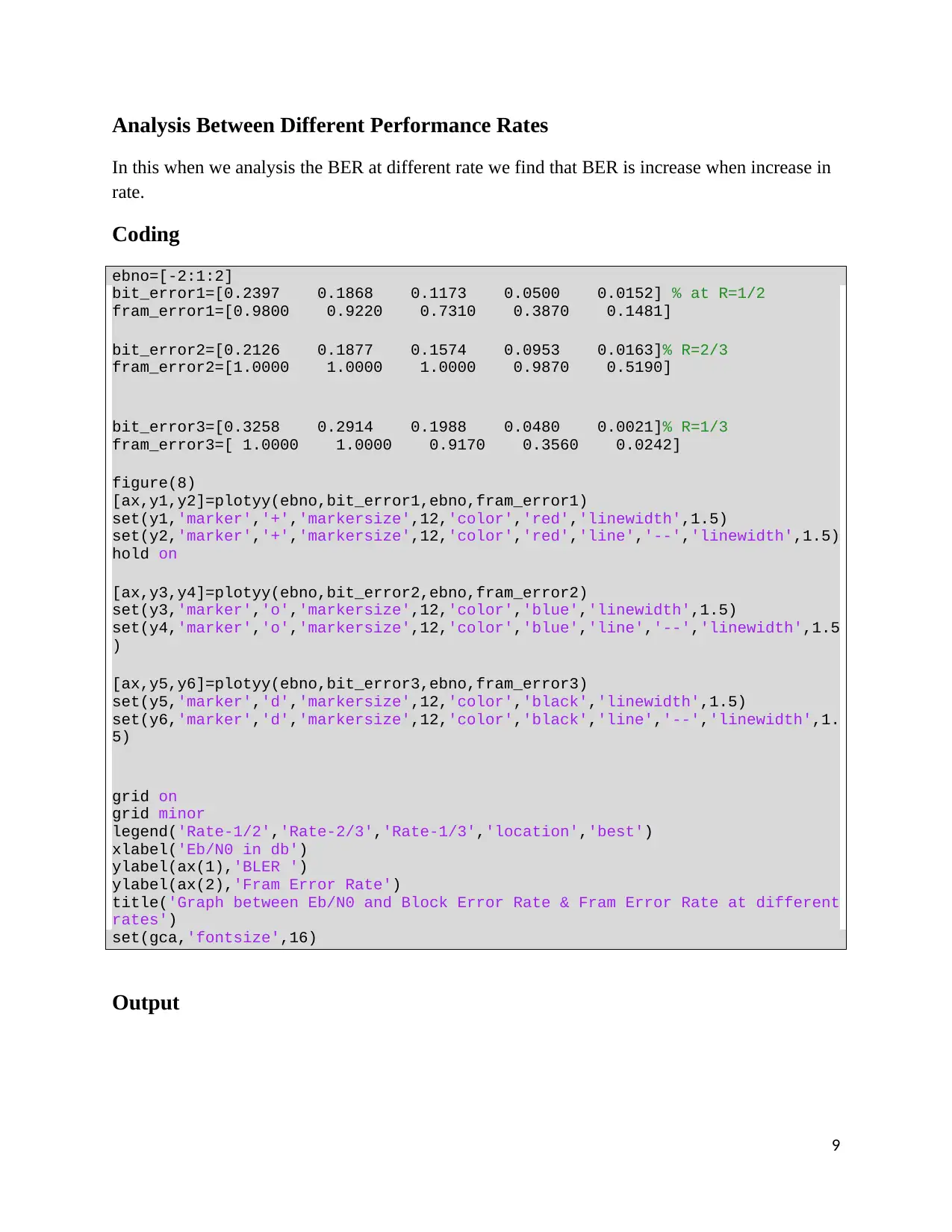
Analysis Between Different Performance Rates
In this when we analysis the BER at different rate we find that BER is increase when increase in
rate.
Coding
ebno=[-2:1:2]
bit_error1=[0.2397 0.1868 0.1173 0.0500 0.0152] % at R=1/2
fram_error1=[0.9800 0.9220 0.7310 0.3870 0.1481]
bit_error2=[0.2126 0.1877 0.1574 0.0953 0.0163]% R=2/3
fram_error2=[1.0000 1.0000 1.0000 0.9870 0.5190]
bit_error3=[0.3258 0.2914 0.1988 0.0480 0.0021]% R=1/3
fram_error3=[ 1.0000 1.0000 0.9170 0.3560 0.0242]
figure(8)
[ax,y1,y2]=plotyy(ebno,bit_error1,ebno,fram_error1)
set(y1,'marker','+','markersize',12,'color','red','linewidth',1.5)
set(y2,'marker','+','markersize',12,'color','red','line','--','linewidth',1.5)
hold on
[ax,y3,y4]=plotyy(ebno,bit_error2,ebno,fram_error2)
set(y3,'marker','o','markersize',12,'color','blue','linewidth',1.5)
set(y4,'marker','o','markersize',12,'color','blue','line','--','linewidth',1.5
)
[ax,y5,y6]=plotyy(ebno,bit_error3,ebno,fram_error3)
set(y5,'marker','d','markersize',12,'color','black','linewidth',1.5)
set(y6,'marker','d','markersize',12,'color','black','line','--','linewidth',1.
5)
grid on
grid minor
legend('Rate-1/2','Rate-2/3','Rate-1/3','location','best')
xlabel('Eb/N0 in db')
ylabel(ax(1),'BLER ')
ylabel(ax(2),'Fram Error Rate')
title('Graph between Eb/N0 and Block Error Rate & Fram Error Rate at different
rates')
set(gca,'fontsize',16)
Output
9
⊘ This is a preview!⊘
Do you want full access?
Subscribe today to unlock all pages.
Trusted by 1+ million students worldwide
-2 -1.5 -1 -0.5 0 0.5 1 1.5 2
0
0.05
0.1
0.15
0.2
0.25
Eb/N0 in db
BLER
Graph between Eb/N0 and Block error Rate & Fram Error Rate at different rates
-2 -1.5 -1 -0.5 0 0.5 1 1.5 20
0.2
0.4
0.6
0.8
1
-2 -1.5 -1 -0.5 0 0.5 1 1.5 20.5
0.6
0.7
0.8
0.9
1
-2 -1.5 -1 -0.5 0 0.5 1 1.5 20
0.2
0.4
0.6
0.8
1
Fram Error Rate
Rate-1/2
Rate-2/3
Rate-1/3
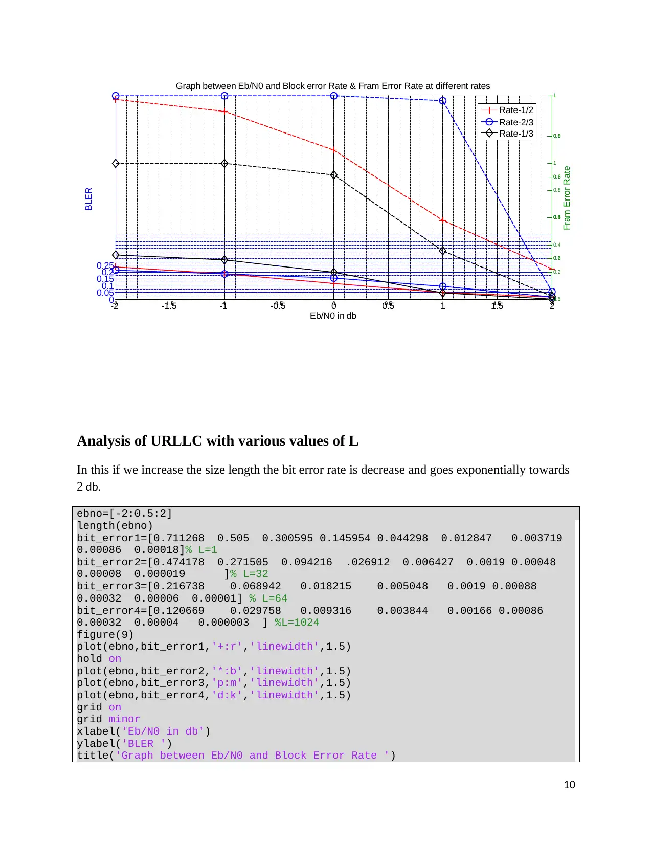
Analysis of URLLC with various values of L
In this if we increase the size length the bit error rate is decrease and goes exponentially towards
2 db.
ebno=[-2:0.5:2]
length(ebno)
bit_error1=[0.711268 0.505 0.300595 0.145954 0.044298 0.012847 0.003719
0.00086 0.00018]% L=1
bit_error2=[0.474178 0.271505 0.094216 .026912 0.006427 0.0019 0.00048
0.00008 0.000019 ]% L=32
bit_error3=[0.216738 0.068942 0.018215 0.005048 0.0019 0.00088
0.00032 0.00006 0.00001] % L=64
bit_error4=[0.120669 0.029758 0.009316 0.003844 0.00166 0.00086
0.00032 0.00004 0.000003 ] %L=1024
figure(9)
plot(ebno,bit_error1,'+:r','linewidth',1.5)
hold on
plot(ebno,bit_error2,'*:b','linewidth',1.5)
plot(ebno,bit_error3,'p:m','linewidth',1.5)
plot(ebno,bit_error4,'d:k','linewidth',1.5)
grid on
grid minor
xlabel('Eb/N0 in db')
ylabel('BLER ')
title('Graph between Eb/N0 and Block Error Rate ')
10
0
0.05
0.1
0.15
0.2
0.25
Eb/N0 in db
BLER
Graph between Eb/N0 and Block error Rate & Fram Error Rate at different rates
-2 -1.5 -1 -0.5 0 0.5 1 1.5 20
0.2
0.4
0.6
0.8
1
-2 -1.5 -1 -0.5 0 0.5 1 1.5 20.5
0.6
0.7
0.8
0.9
1
-2 -1.5 -1 -0.5 0 0.5 1 1.5 20
0.2
0.4
0.6
0.8
1
Fram Error Rate
Rate-1/2
Rate-2/3
Rate-1/3
Analysis of URLLC with various values of L
In this if we increase the size length the bit error rate is decrease and goes exponentially towards
2 db.
ebno=[-2:0.5:2]
length(ebno)
bit_error1=[0.711268 0.505 0.300595 0.145954 0.044298 0.012847 0.003719
0.00086 0.00018]% L=1
bit_error2=[0.474178 0.271505 0.094216 .026912 0.006427 0.0019 0.00048
0.00008 0.000019 ]% L=32
bit_error3=[0.216738 0.068942 0.018215 0.005048 0.0019 0.00088
0.00032 0.00006 0.00001] % L=64
bit_error4=[0.120669 0.029758 0.009316 0.003844 0.00166 0.00086
0.00032 0.00004 0.000003 ] %L=1024
figure(9)
plot(ebno,bit_error1,'+:r','linewidth',1.5)
hold on
plot(ebno,bit_error2,'*:b','linewidth',1.5)
plot(ebno,bit_error3,'p:m','linewidth',1.5)
plot(ebno,bit_error4,'d:k','linewidth',1.5)
grid on
grid minor
xlabel('Eb/N0 in db')
ylabel('BLER ')
title('Graph between Eb/N0 and Block Error Rate ')
10
Paraphrase This Document
Need a fresh take? Get an instant paraphrase of this document with our AI Paraphraser
legend('L=1','L=32','L=64','L=1024')
Output
-2 -1.5 -1 -0.5 0 0.5 1 1.5 2
0
0.1
0.2
0.3
0.4
0.5
0.6
0.7
0.8
Eb/N0 in db
BLER
Graph between Eb/N0 and Block Error Rate
L=1
L=32
L=64
L=1024
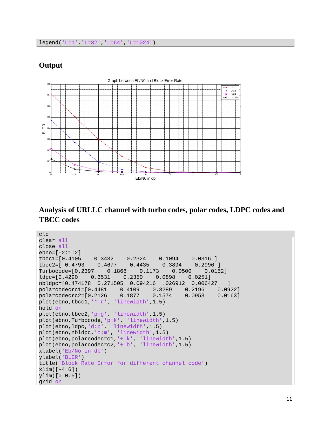
Analysis of URLLC channel with turbo codes, polar codes, LDPC codes and
TBCC codes
clc
clear all
close all
ebno=[-2:1:2]
tbcc1=[0.4105 0.3432 0.2324 0.1094 0.0316 ]
tbcc2=[ 0.4793 0.4677 0.4435 0.3894 0.2996 ]
Turbocode=[0.2397 0.1868 0.1173 0.0500 0.0152]
ldpc=[0.4290 0.3531 0.2350 0.0898 0.0251]
nbldpc=[0.474178 0.271505 0.094216 .026912 0.006427 ]
polarcodecrc1=[0.4481 0.4109 0.3289 0.2196 0.0922]
polarcodecrc2=[0.2126 0.1877 0.1574 0.0953 0.0163]
plot(ebno,tbcc1,'*:r', 'linewidth',1.5)
hold on
plot(ebno,tbcc2,'p:g', 'linewidth',1.5)
plot(ebno,Turbocode,'p:k', 'linewidth',1.5)
plot(ebno,ldpc,'d:b', 'linewidth',1.5)
plot(ebno,nbldpc,'o:m', 'linewidth',1.5)
plot(ebno,polarcodecrc1,'+:k', 'linewidth',1.5)
plot(ebno,polarcodecrc2,'+:b', 'linewidth',1.5)
xlabel('Eb/No in db')
ylabel('BLER')
title('Block Rate Error for different channel code')
xlim([-4 6])
ylim([0 0.5])
grid on
11
Output
-2 -1.5 -1 -0.5 0 0.5 1 1.5 2
0
0.1
0.2
0.3
0.4
0.5
0.6
0.7
0.8
Eb/N0 in db
BLER
Graph between Eb/N0 and Block Error Rate
L=1
L=32
L=64
L=1024
Analysis of URLLC channel with turbo codes, polar codes, LDPC codes and
TBCC codes
clc
clear all
close all
ebno=[-2:1:2]
tbcc1=[0.4105 0.3432 0.2324 0.1094 0.0316 ]
tbcc2=[ 0.4793 0.4677 0.4435 0.3894 0.2996 ]
Turbocode=[0.2397 0.1868 0.1173 0.0500 0.0152]
ldpc=[0.4290 0.3531 0.2350 0.0898 0.0251]
nbldpc=[0.474178 0.271505 0.094216 .026912 0.006427 ]
polarcodecrc1=[0.4481 0.4109 0.3289 0.2196 0.0922]
polarcodecrc2=[0.2126 0.1877 0.1574 0.0953 0.0163]
plot(ebno,tbcc1,'*:r', 'linewidth',1.5)
hold on
plot(ebno,tbcc2,'p:g', 'linewidth',1.5)
plot(ebno,Turbocode,'p:k', 'linewidth',1.5)
plot(ebno,ldpc,'d:b', 'linewidth',1.5)
plot(ebno,nbldpc,'o:m', 'linewidth',1.5)
plot(ebno,polarcodecrc1,'+:k', 'linewidth',1.5)
plot(ebno,polarcodecrc2,'+:b', 'linewidth',1.5)
xlabel('Eb/No in db')
ylabel('BLER')
title('Block Rate Error for different channel code')
xlim([-4 6])
ylim([0 0.5])
grid on
11
grid minor
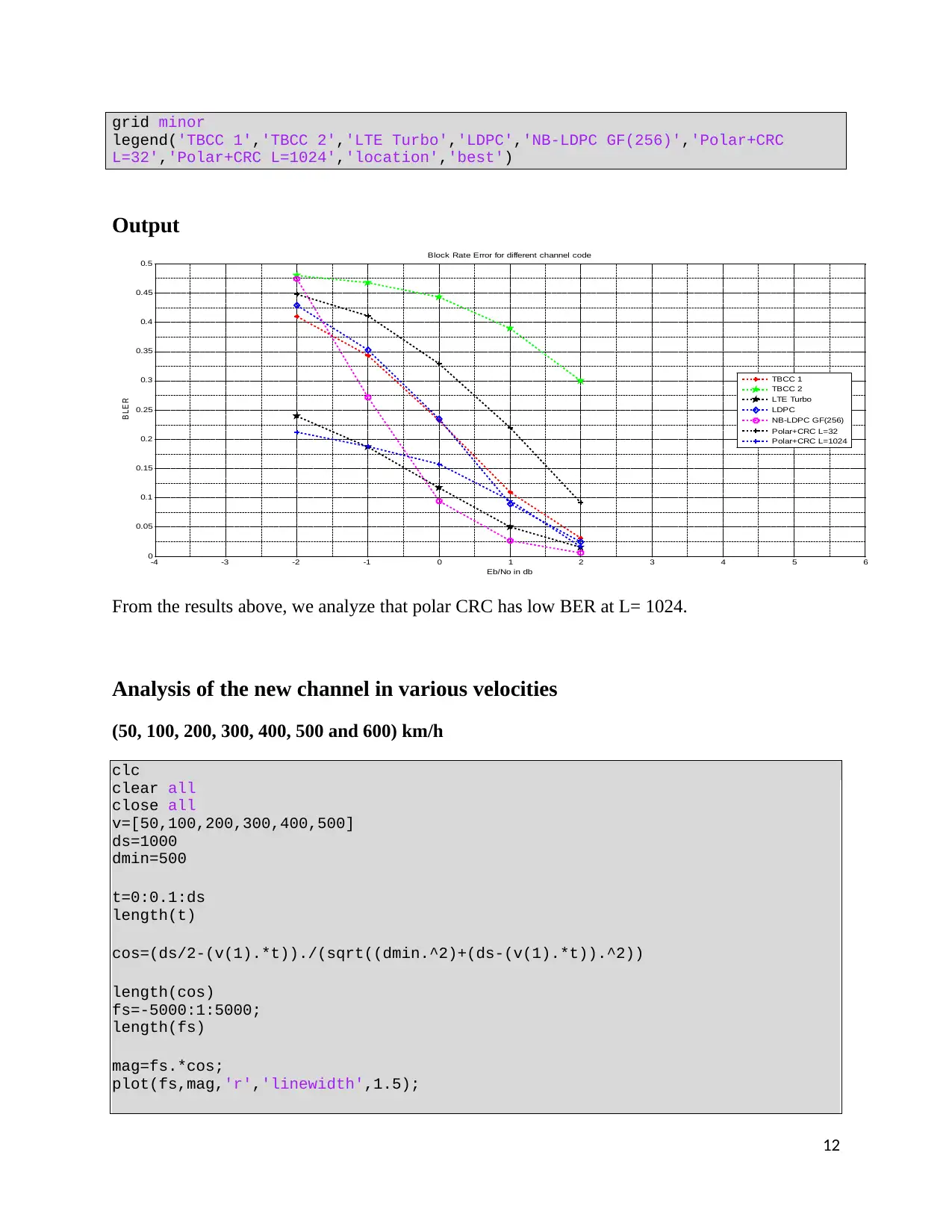
legend('TBCC 1','TBCC 2','LTE Turbo','LDPC','NB-LDPC GF(256)','Polar+CRC
L=32','Polar+CRC L=1024','location','best')
Output
-4 -3 -2 -1 0 1 2 3 4 5 6
0
0.05
0.1
0.15
0.2
0.25
0.3
0.35
0.4
0.45
0.5
Eb/No in db
B LE R
Block Rate Error for different channel code
TBCC 1
TBCC 2
LTE Turbo
LDPC
NB-LDPC GF(256)
Polar+CRC L=32
Polar+CRC L=1024
From the results above, we analyze that polar CRC has low BER at L= 1024.
Analysis of the new channel in various velocities
(50, 100, 200, 300, 400, 500 and 600) km/h
clc
clear all
close all
v=[50,100,200,300,400,500]
ds=1000
dmin=500
t=0:0.1:ds
length(t)
cos=(ds/2-(v(1).*t))./(sqrt((dmin.^2)+(ds-(v(1).*t)).^2))
length(cos)
fs=-5000:1:5000;
length(fs)
mag=fs.*cos;
plot(fs,mag,'r','linewidth',1.5);
12
⊘ This is a preview!⊘
Do you want full access?
Subscribe today to unlock all pages.
Trusted by 1+ million students worldwide
1 out of 15
Your All-in-One AI-Powered Toolkit for Academic Success.
+13062052269
info@desklib.com
Available 24*7 on WhatsApp / Email
![[object Object]](/_next/static/media/star-bottom.7253800d.svg)
Unlock your academic potential
Copyright © 2020–2026 A2Z Services. All Rights Reserved. Developed and managed by ZUCOL.