Statistical Report: Analyzing US Worker Data - Wages, Education, 2018
VerifiedAdded on 2023/06/12
|12
|1801
|73
Report
AI Summary
This report analyzes data related to US workers in 2018, focusing on wages and education levels obtained from the Economic Web Institute. It includes descriptive statistics such as mean, median, standard deviation, and frequency distributions for both wages and education. Hypothesis testing is conducted to determine if the proportion of tertiary education has increased since 2017 and whether the average wage in 2018 differs from that of 2017. Additionally, the report explores real estate prices in Sydney suburbs, comparing house prices in Alexandria and Annadale using statistical methods to inform a potential property purchase. Desklib provides similar solved assignments and resources for students.
Running head: BUSINESS DECISION MAKING
Business Decision Making
Name of the Student:
Name of the University:
Author’s Note:
Business Decision Making
Name of the Student:
Name of the University:
Author’s Note:
Paraphrase This Document
Need a fresh take? Get an instant paraphrase of this document with our AI Paraphraser
1BUSINESS DECISION MAKING
Table of Contents
Background:...............................................................................................................................2
Answer 1....................................................................................................................................2
Answer 1.1.............................................................................................................................2
Answer 1.2.............................................................................................................................2
Answer 1.3.............................................................................................................................6
Answer 1.4.............................................................................................................................7
Answer 2....................................................................................................................................8
Answer 2.1.............................................................................................................................8
Answer 2.2.............................................................................................................................8
Answer 2.3.............................................................................................................................8
Answer 2.4.............................................................................................................................9
References:...............................................................................................................................10
2BUSINESS DECISION MAKING
Background:
It is assumed that Economic Web Institute conducted a research on wages of US workers in
2018. The samples have the data of 536 workers and it involves various information about the
workers. Note that, “KADD” add-ins helped to analyse the data set properly.
Answer 1.
Answer 1.1.
Economics web Institute is interested in the workers of United States in the session 2018. For
analysis purpose, we mainly have granted two variables about the workers that are “wage”
and “education level”.
Answer 1.2.
Wages:
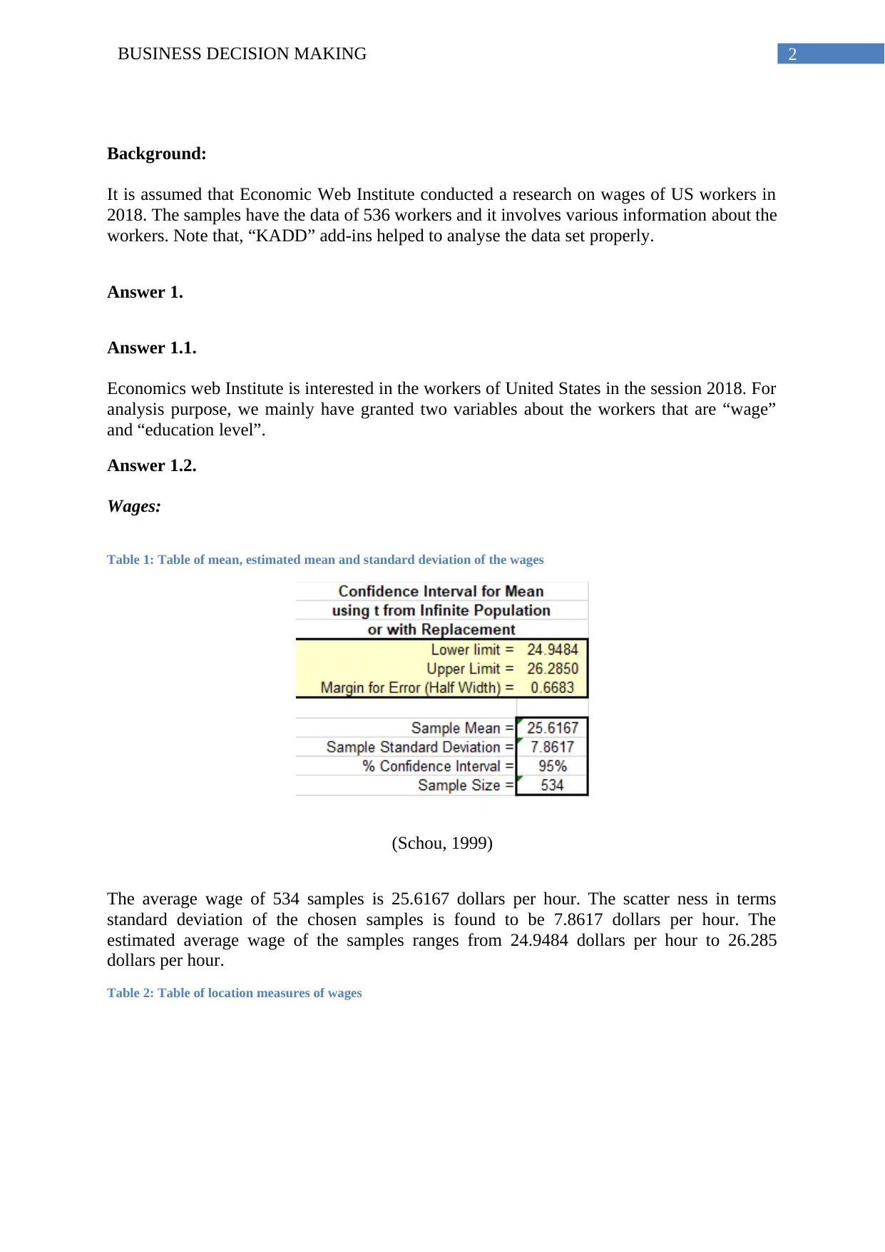
Table 1: Table of mean, estimated mean and standard deviation of the wages
(Schou, 1999)
The average wage of 534 samples is 25.6167 dollars per hour. The scatter ness in terms
standard deviation of the chosen samples is found to be 7.8617 dollars per hour. The
estimated average wage of the samples ranges from 24.9484 dollars per hour to 26.285
dollars per hour.
Table 2: Table of location measures of wages
Background:
It is assumed that Economic Web Institute conducted a research on wages of US workers in
2018. The samples have the data of 536 workers and it involves various information about the
workers. Note that, “KADD” add-ins helped to analyse the data set properly.
Answer 1.
Answer 1.1.
Economics web Institute is interested in the workers of United States in the session 2018. For
analysis purpose, we mainly have granted two variables about the workers that are “wage”
and “education level”.
Answer 1.2.
Wages:
Table 1: Table of mean, estimated mean and standard deviation of the wages
(Schou, 1999)
The average wage of 534 samples is 25.6167 dollars per hour. The scatter ness in terms
standard deviation of the chosen samples is found to be 7.8617 dollars per hour. The
estimated average wage of the samples ranges from 24.9484 dollars per hour to 26.285
dollars per hour.
Table 2: Table of location measures of wages
⊘ This is a preview!⊘
Do you want full access?
Subscribe today to unlock all pages.
Trusted by 1+ million students worldwide
3BUSINESS DECISION MAKING
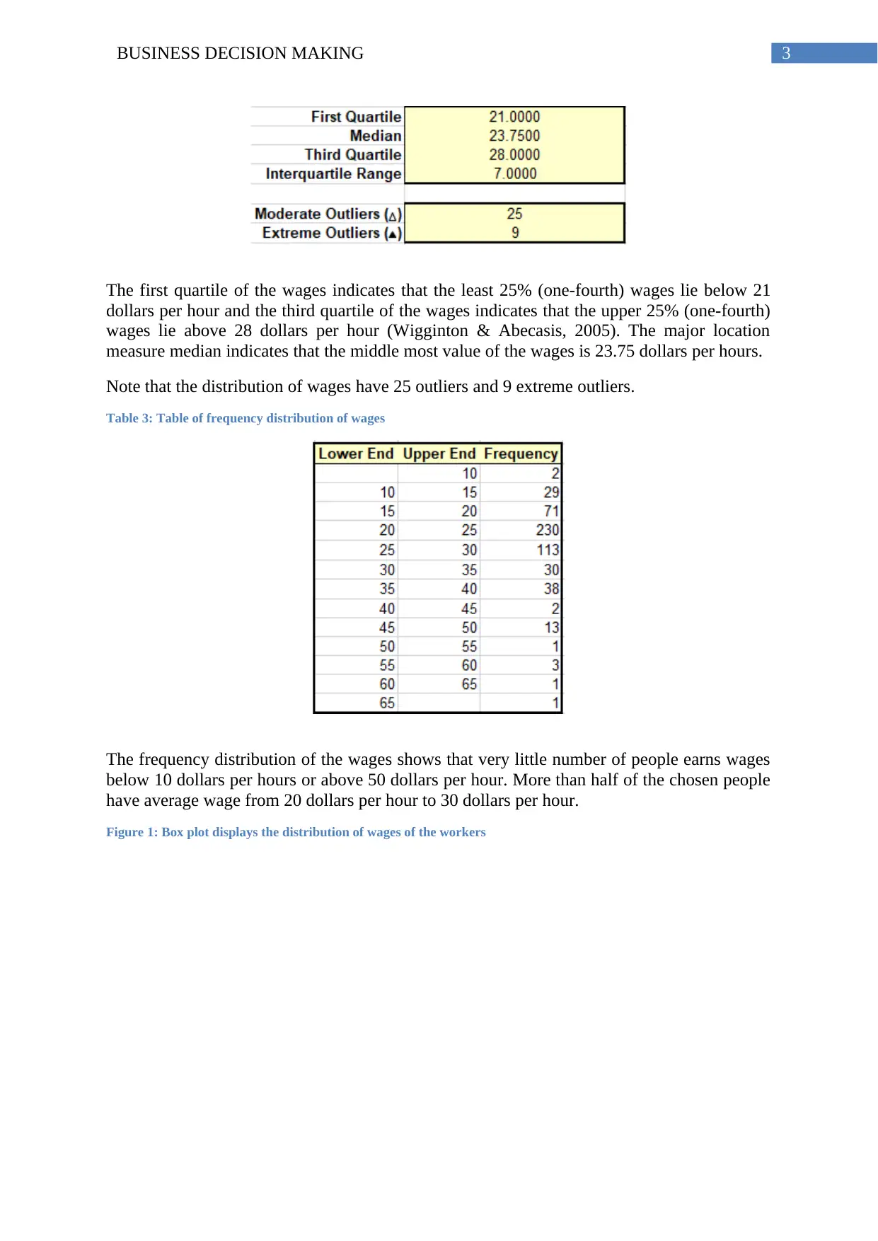
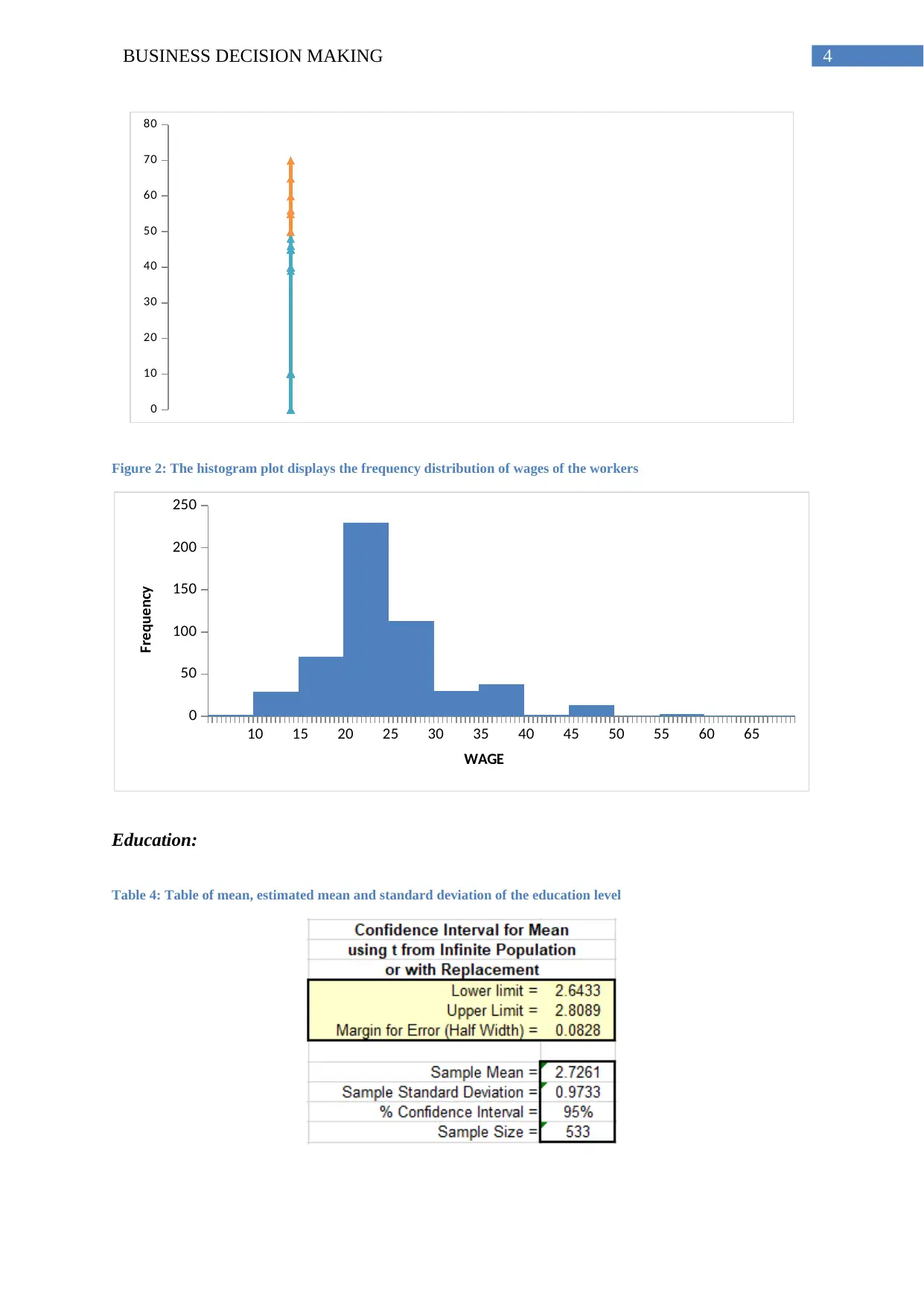
The first quartile of the wages indicates that the least 25% (one-fourth) wages lie below 21
dollars per hour and the third quartile of the wages indicates that the upper 25% (one-fourth)
wages lie above 28 dollars per hour (Wigginton & Abecasis, 2005). The major location
measure median indicates that the middle most value of the wages is 23.75 dollars per hours.
Note that the distribution of wages have 25 outliers and 9 extreme outliers.
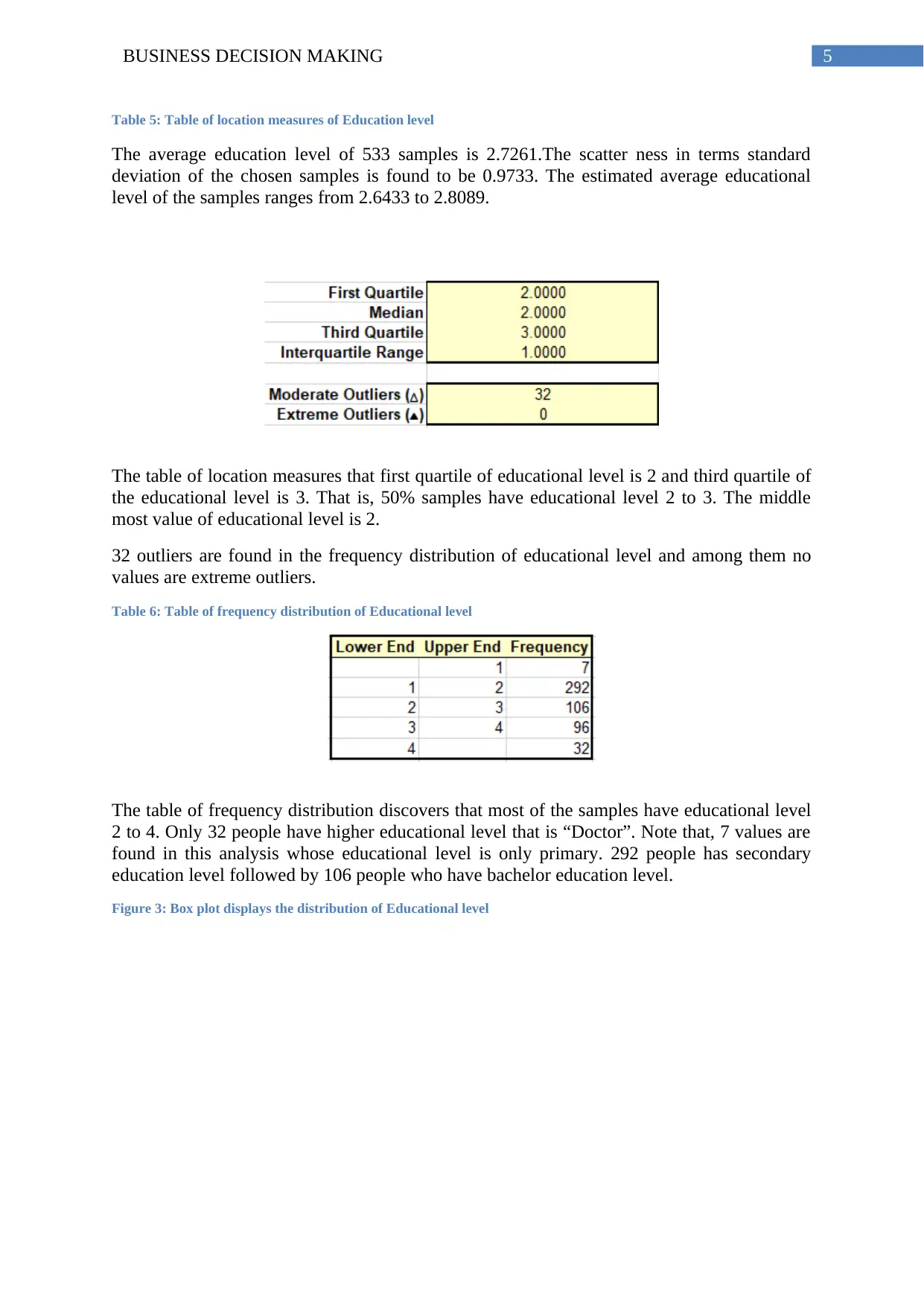
Table 3: Table of frequency distribution of wages
The frequency distribution of the wages shows that very little number of people earns wages
below 10 dollars per hours or above 50 dollars per hour. More than half of the chosen people
have average wage from 20 dollars per hour to 30 dollars per hour.
Figure 1: Box plot displays the distribution of wages of the workers
The first quartile of the wages indicates that the least 25% (one-fourth) wages lie below 21
dollars per hour and the third quartile of the wages indicates that the upper 25% (one-fourth)
wages lie above 28 dollars per hour (Wigginton & Abecasis, 2005). The major location
measure median indicates that the middle most value of the wages is 23.75 dollars per hours.
Note that the distribution of wages have 25 outliers and 9 extreme outliers.
Table 3: Table of frequency distribution of wages
The frequency distribution of the wages shows that very little number of people earns wages
below 10 dollars per hours or above 50 dollars per hour. More than half of the chosen people
have average wage from 20 dollars per hour to 30 dollars per hour.
Figure 1: Box plot displays the distribution of wages of the workers
Paraphrase This Document
Need a fresh take? Get an instant paraphrase of this document with our AI Paraphraser
4BUSINESS DECISION MAKING
0
10
20
30
40
50
60
70
80
Figure 2: The histogram plot displays the frequency distribution of wages of the workers
10 15 20 25 30 35 40 45 50 55 60 65
0
50
100
150
200
250
WAGE
Frequency
Education:
Table 4: Table of mean, estimated mean and standard deviation of the education level
0
10
20
30
40
50
60
70
80
Figure 2: The histogram plot displays the frequency distribution of wages of the workers
10 15 20 25 30 35 40 45 50 55 60 65
0
50
100
150
200
250
WAGE
Frequency
Education:
Table 4: Table of mean, estimated mean and standard deviation of the education level
5BUSINESS DECISION MAKING
Table 5: Table of location measures of Education level
The average education level of 533 samples is 2.7261.The scatter ness in terms standard
deviation of the chosen samples is found to be 0.9733. The estimated average educational
level of the samples ranges from 2.6433 to 2.8089.
The table of location measures that first quartile of educational level is 2 and third quartile of
the educational level is 3. That is, 50% samples have educational level 2 to 3. The middle
most value of educational level is 2.
32 outliers are found in the frequency distribution of educational level and among them no
values are extreme outliers.
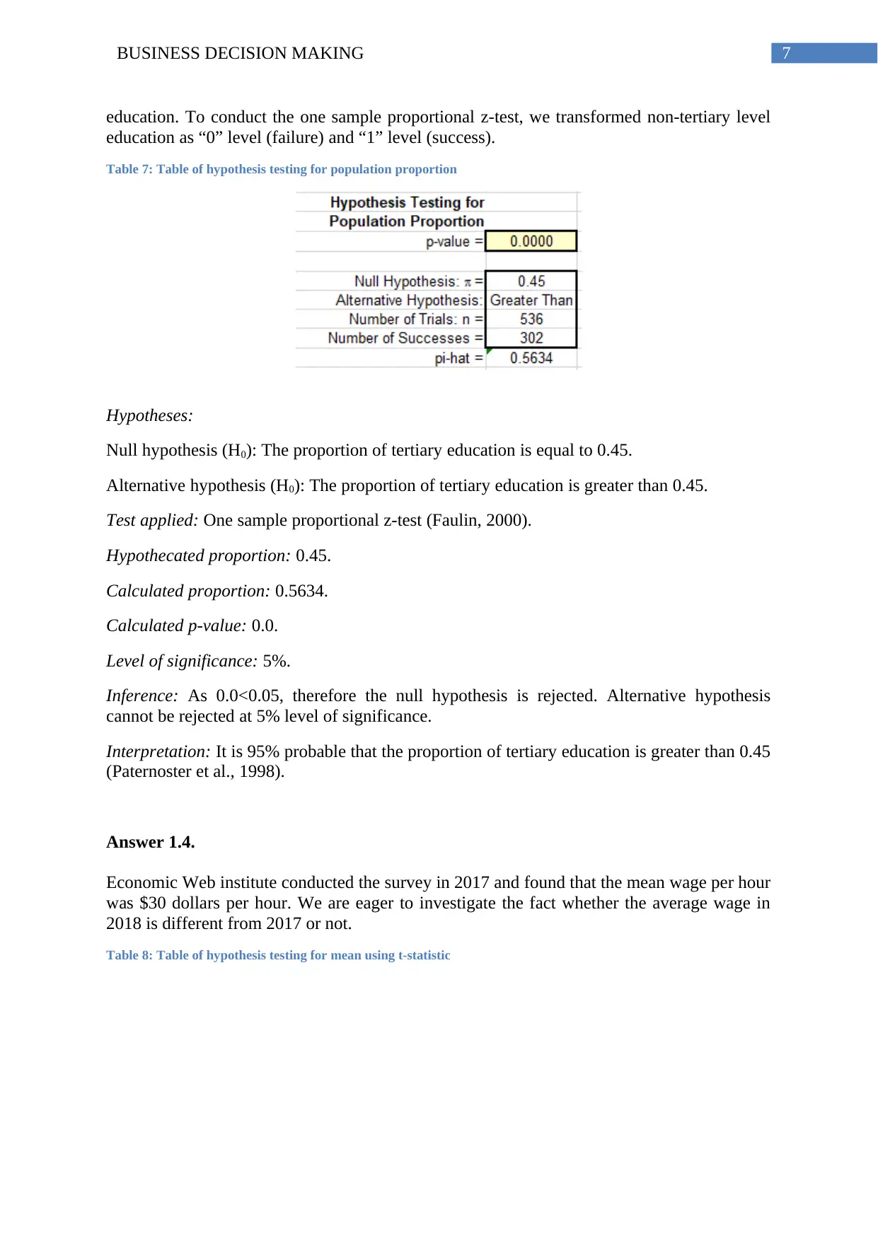
Table 6: Table of frequency distribution of Educational level
The table of frequency distribution discovers that most of the samples have educational level
2 to 4. Only 32 people have higher educational level that is “Doctor”. Note that, 7 values are
found in this analysis whose educational level is only primary. 292 people has secondary
education level followed by 106 people who have bachelor education level.
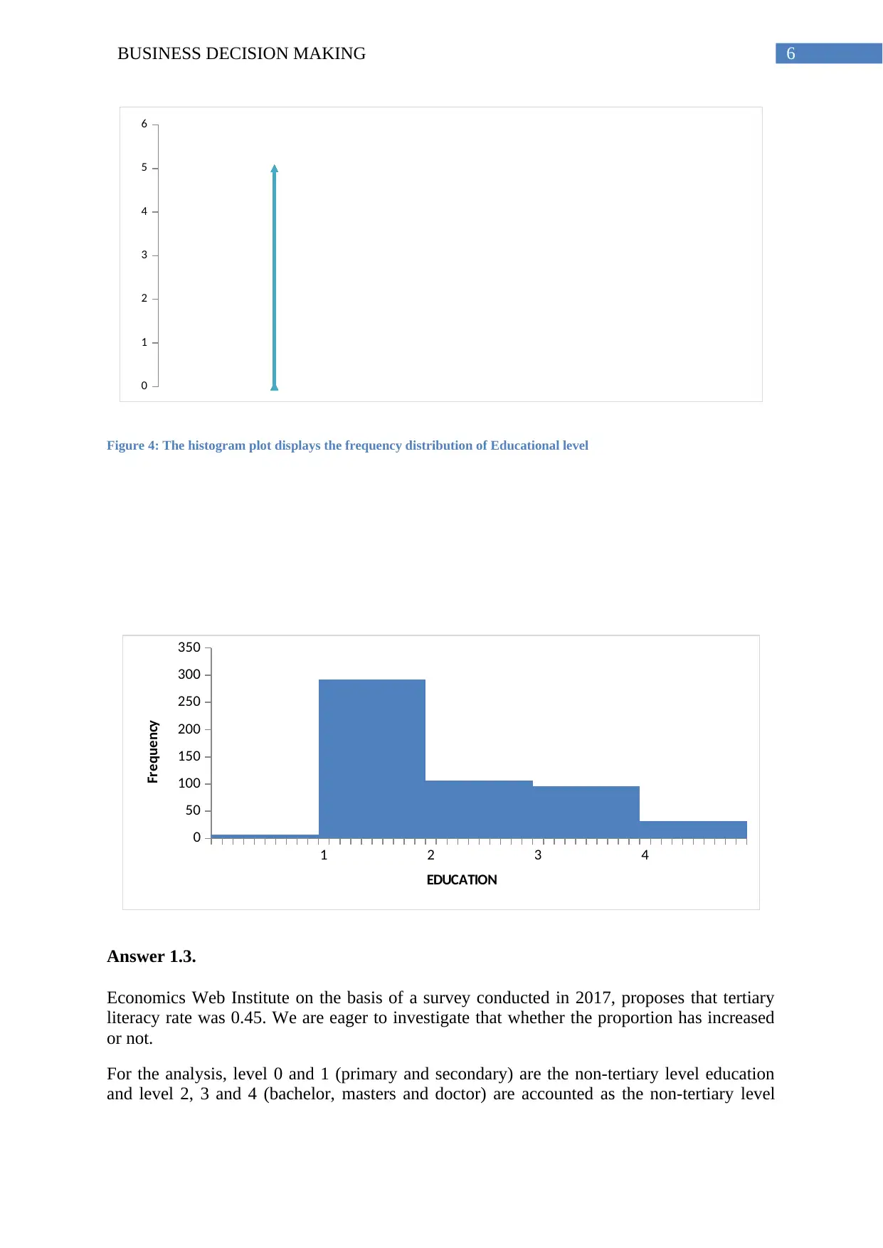
Figure 3: Box plot displays the distribution of Educational level
Table 5: Table of location measures of Education level
The average education level of 533 samples is 2.7261.The scatter ness in terms standard
deviation of the chosen samples is found to be 0.9733. The estimated average educational
level of the samples ranges from 2.6433 to 2.8089.
The table of location measures that first quartile of educational level is 2 and third quartile of
the educational level is 3. That is, 50% samples have educational level 2 to 3. The middle
most value of educational level is 2.
32 outliers are found in the frequency distribution of educational level and among them no
values are extreme outliers.
Table 6: Table of frequency distribution of Educational level
The table of frequency distribution discovers that most of the samples have educational level
2 to 4. Only 32 people have higher educational level that is “Doctor”. Note that, 7 values are
found in this analysis whose educational level is only primary. 292 people has secondary
education level followed by 106 people who have bachelor education level.
Figure 3: Box plot displays the distribution of Educational level
⊘ This is a preview!⊘
Do you want full access?
Subscribe today to unlock all pages.
Trusted by 1+ million students worldwide
6BUSINESS DECISION MAKING
0
1
2
3
4
5
6
Figure 4: The histogram plot displays the frequency distribution of Educational level
1 2 3 4
0
50
100
150
200
250
300
350
EDUCATION
Frequency
Answer 1.3.
Economics Web Institute on the basis of a survey conducted in 2017, proposes that tertiary
literacy rate was 0.45. We are eager to investigate that whether the proportion has increased
or not.
For the analysis, level 0 and 1 (primary and secondary) are the non-tertiary level education
and level 2, 3 and 4 (bachelor, masters and doctor) are accounted as the non-tertiary level
0
1
2
3
4
5
6
Figure 4: The histogram plot displays the frequency distribution of Educational level
1 2 3 4
0
50
100
150
200
250
300
350
EDUCATION
Frequency
Answer 1.3.
Economics Web Institute on the basis of a survey conducted in 2017, proposes that tertiary
literacy rate was 0.45. We are eager to investigate that whether the proportion has increased
or not.
For the analysis, level 0 and 1 (primary and secondary) are the non-tertiary level education
and level 2, 3 and 4 (bachelor, masters and doctor) are accounted as the non-tertiary level
Paraphrase This Document
Need a fresh take? Get an instant paraphrase of this document with our AI Paraphraser
7BUSINESS DECISION MAKING
education. To conduct the one sample proportional z-test, we transformed non-tertiary level
education as “0” level (failure) and “1” level (success).
Table 7: Table of hypothesis testing for population proportion
Hypotheses:
Null hypothesis (H0): The proportion of tertiary education is equal to 0.45.
Alternative hypothesis (H0): The proportion of tertiary education is greater than 0.45.
Test applied: One sample proportional z-test (Faulin, 2000).
Hypothecated proportion: 0.45.
Calculated proportion: 0.5634.
Calculated p-value: 0.0.
Level of significance: 5%.
Inference: As 0.0<0.05, therefore the null hypothesis is rejected. Alternative hypothesis
cannot be rejected at 5% level of significance.
Interpretation: It is 95% probable that the proportion of tertiary education is greater than 0.45
(Paternoster et al., 1998).
Answer 1.4.
Economic Web institute conducted the survey in 2017 and found that the mean wage per hour
was $30 dollars per hour. We are eager to investigate the fact whether the average wage in
2018 is different from 2017 or not.
Table 8: Table of hypothesis testing for mean using t-statistic
8BUSINESS DECISION MAKING
Hypotheses:
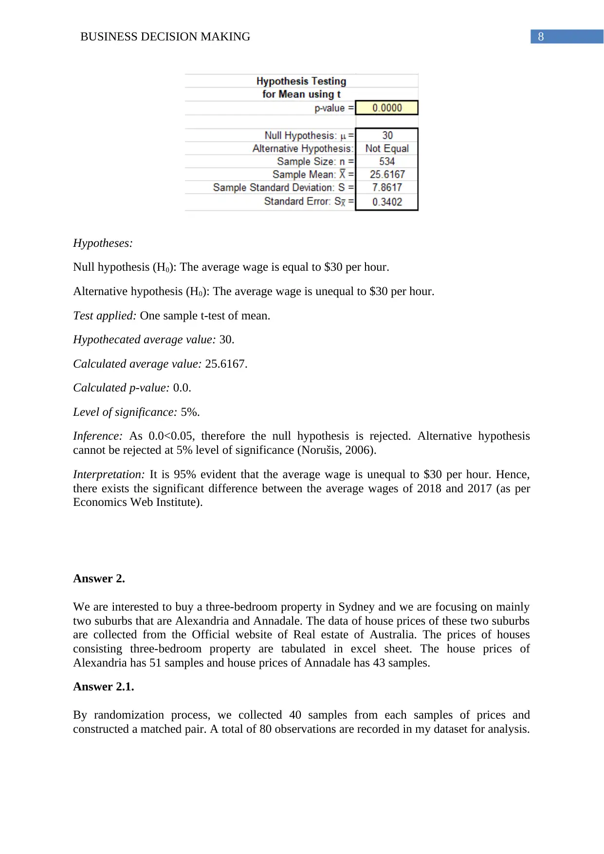
Null hypothesis (H0): The average wage is equal to $30 per hour.
Alternative hypothesis (H0): The average wage is unequal to $30 per hour.
Test applied: One sample t-test of mean.
Hypothecated average value: 30.
Calculated average value: 25.6167.
Calculated p-value: 0.0.
Level of significance: 5%.
Inference: As 0.0<0.05, therefore the null hypothesis is rejected. Alternative hypothesis
cannot be rejected at 5% level of significance (Norušis, 2006).
Interpretation: It is 95% evident that the average wage is unequal to $30 per hour. Hence,
there exists the significant difference between the average wages of 2018 and 2017 (as per
Economics Web Institute).
Answer 2.
We are interested to buy a three-bedroom property in Sydney and we are focusing on mainly
two suburbs that are Alexandria and Annadale. The data of house prices of these two suburbs
are collected from the Official website of Real estate of Australia. The prices of houses
consisting three-bedroom property are tabulated in excel sheet. The house prices of
Alexandria has 51 samples and house prices of Annadale has 43 samples.
Answer 2.1.
By randomization process, we collected 40 samples from each samples of prices and
constructed a matched pair. A total of 80 observations are recorded in my dataset for analysis.
Hypotheses:
Null hypothesis (H0): The average wage is equal to $30 per hour.
Alternative hypothesis (H0): The average wage is unequal to $30 per hour.
Test applied: One sample t-test of mean.
Hypothecated average value: 30.
Calculated average value: 25.6167.
Calculated p-value: 0.0.
Level of significance: 5%.
Inference: As 0.0<0.05, therefore the null hypothesis is rejected. Alternative hypothesis
cannot be rejected at 5% level of significance (Norušis, 2006).
Interpretation: It is 95% evident that the average wage is unequal to $30 per hour. Hence,
there exists the significant difference between the average wages of 2018 and 2017 (as per
Economics Web Institute).
Answer 2.
We are interested to buy a three-bedroom property in Sydney and we are focusing on mainly
two suburbs that are Alexandria and Annadale. The data of house prices of these two suburbs
are collected from the Official website of Real estate of Australia. The prices of houses
consisting three-bedroom property are tabulated in excel sheet. The house prices of
Alexandria has 51 samples and house prices of Annadale has 43 samples.
Answer 2.1.
By randomization process, we collected 40 samples from each samples of prices and
constructed a matched pair. A total of 80 observations are recorded in my dataset for analysis.
⊘ This is a preview!⊘
Do you want full access?
Subscribe today to unlock all pages.
Trusted by 1+ million students worldwide
9BUSINESS DECISION MAKING
Answer 2.2.
The populations that we are interested in are the prices of three-bedroom houses located in
the two suburbs of Sydney named Alexandria and Annadale.
Answer 2.3.
2.3.1. Estimation:
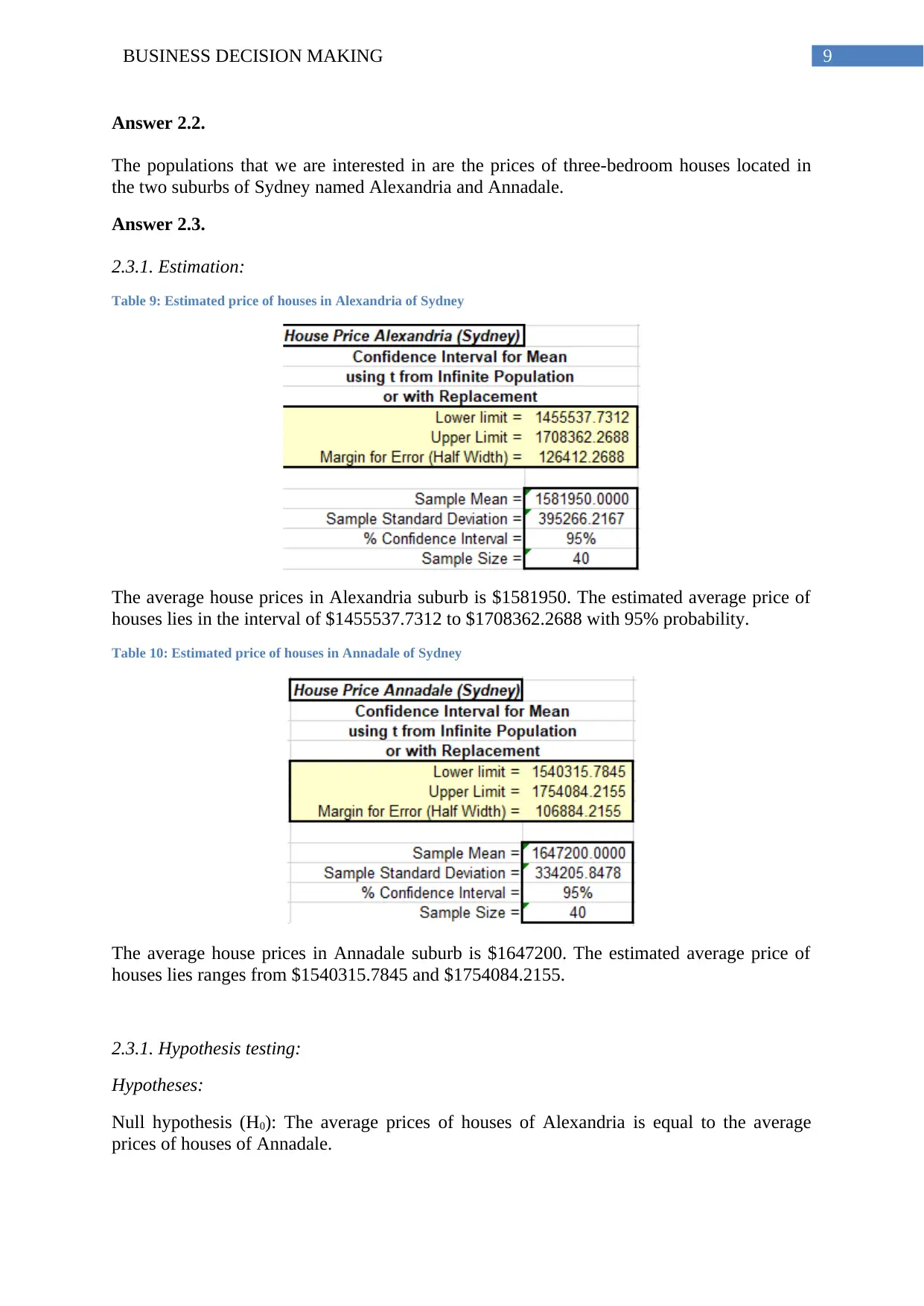
Table 9: Estimated price of houses in Alexandria of Sydney
The average house prices in Alexandria suburb is $1581950. The estimated average price of
houses lies in the interval of $1455537.7312 to $1708362.2688 with 95% probability.
Table 10: Estimated price of houses in Annadale of Sydney
The average house prices in Annadale suburb is $1647200. The estimated average price of
houses lies ranges from $1540315.7845 and $1754084.2155.
2.3.1. Hypothesis testing:
Hypotheses:
Null hypothesis (H0): The average prices of houses of Alexandria is equal to the average
prices of houses of Annadale.
Answer 2.2.
The populations that we are interested in are the prices of three-bedroom houses located in
the two suburbs of Sydney named Alexandria and Annadale.
Answer 2.3.
2.3.1. Estimation:
Table 9: Estimated price of houses in Alexandria of Sydney
The average house prices in Alexandria suburb is $1581950. The estimated average price of
houses lies in the interval of $1455537.7312 to $1708362.2688 with 95% probability.
Table 10: Estimated price of houses in Annadale of Sydney
The average house prices in Annadale suburb is $1647200. The estimated average price of
houses lies ranges from $1540315.7845 and $1754084.2155.
2.3.1. Hypothesis testing:
Hypotheses:
Null hypothesis (H0): The average prices of houses of Alexandria is equal to the average
prices of houses of Annadale.
Paraphrase This Document
Need a fresh take? Get an instant paraphrase of this document with our AI Paraphraser
10BUSINESS DECISION MAKING
Alternative hypothesis (H0): The average prices of houses of Alexandria is unequal to the
average prices of houses of Annadale.
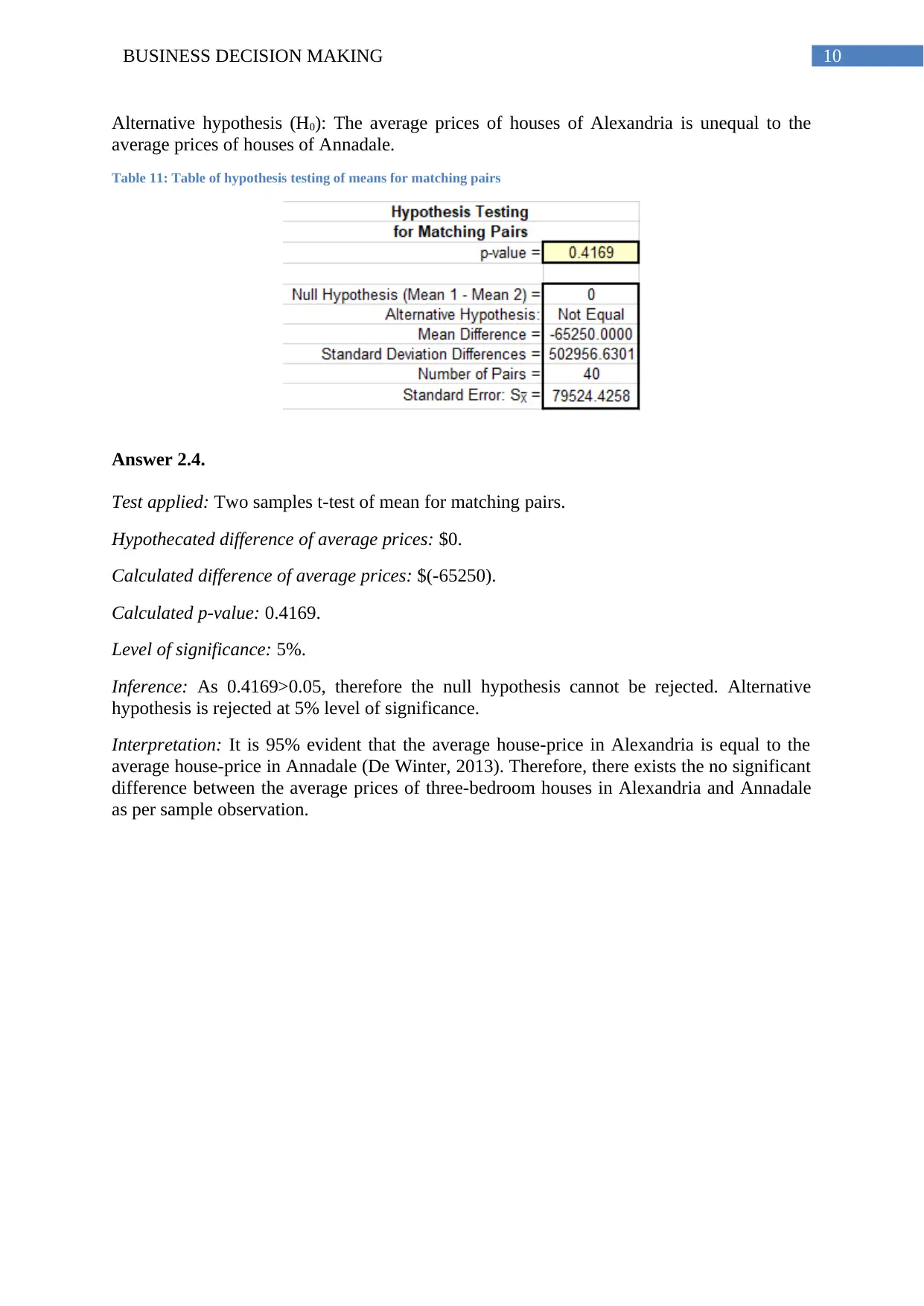
Table 11: Table of hypothesis testing of means for matching pairs
Answer 2.4.
Test applied: Two samples t-test of mean for matching pairs.
Hypothecated difference of average prices: $0.
Calculated difference of average prices: $(-65250).
Calculated p-value: 0.4169.
Level of significance: 5%.
Inference: As 0.4169>0.05, therefore the null hypothesis cannot be rejected. Alternative
hypothesis is rejected at 5% level of significance.
Interpretation: It is 95% evident that the average house-price in Alexandria is equal to the
average house-price in Annadale (De Winter, 2013). Therefore, there exists the no significant
difference between the average prices of three-bedroom houses in Alexandria and Annadale
as per sample observation.
Alternative hypothesis (H0): The average prices of houses of Alexandria is unequal to the
average prices of houses of Annadale.
Table 11: Table of hypothesis testing of means for matching pairs
Answer 2.4.
Test applied: Two samples t-test of mean for matching pairs.
Hypothecated difference of average prices: $0.
Calculated difference of average prices: $(-65250).
Calculated p-value: 0.4169.
Level of significance: 5%.
Inference: As 0.4169>0.05, therefore the null hypothesis cannot be rejected. Alternative
hypothesis is rejected at 5% level of significance.
Interpretation: It is 95% evident that the average house-price in Alexandria is equal to the
average house-price in Annadale (De Winter, 2013). Therefore, there exists the no significant
difference between the average prices of three-bedroom houses in Alexandria and Annadale
as per sample observation.
11BUSINESS DECISION MAKING
References:
De Winter, J. C. (2013). Using the Student's t-test with extremely small sample
sizes. Practical Assessment, Research & Evaluation, 18(10).
Faulin, J. (2000). Data, Statistics, and Decision Models with Excel.
Norušis, M. J. (2006). SPSS 14.0 guide to data analysis. Upper Saddle River, NJ: Prentice
Hall.
Paternoster, R., Brame, R., Mazerolle, P., & Piquero, A. (1998). Using the correct statistical
test for the equality of regression coefficients. Criminology, 36(4), 859-866.
Schou, S. B. (1999). Data, Statistics, and Decision Models with Excel. The American
Statistician, 53(4), 389.
Wigginton, J. E., & Abecasis, G. R. (2005). PEDSTATS: descriptive statistics, graphics and
quality assessment for gene mapping data. Bioinformatics, 21(16), 3445-3447.
⊘ This is a preview!⊘
Do you want full access?
Subscribe today to unlock all pages.
Trusted by 1+ million students worldwide
1 out of 12
Related Documents


Your All-in-One AI-Powered Toolkit for Academic Success.
+13062052269
info@desklib.com
Available 24*7 on WhatsApp / Email
![[object Object]](/_next/static/media/star-bottom.7253800d.svg)
Unlock your academic potential
Copyright © 2020–2026 A2Z Services. All Rights Reserved. Developed and managed by ZUCOL.