Estimation of Crimes in the USA in 1990-92 Regression Model Analysis
VerifiedAdded on 2023/04/22
|31
|5388
|248
Report
AI Summary
This report employs linear and distribution-based regression models to estimate crime rates (crm1000) in the USA during 1990-92. It addresses the issue of crime calculation based on limited offenses when the population is less than the infringement percentage. The study examines crime extent across 440 county districts in four US states, comparing Multiple Linear Regression (MLR) with Poisson and Negative Binomial regression models. The analysis reveals that the Negative Binomial Model provides a better fit for estimating crm1000. The methodology includes correlation analysis, outlier detection, and stepwise MLR, alongside Poisson and Negative Binomial regressions, using an 80:20 training/testing data split of US county demographic information from 1990-92 to ensure prediction accuracy.

RUNNING HEAD: ESTIMATION OF CRIMES IN THE USA IN 1990-92 – A COMPARATIVE ANALYSIS OF
MULTIPLE LINEAR REGRESSION WITH POISSON/NEGATIVE BINOMIAL REGRESSION MODELLING
Estimation of Crimes in the USA in 1990-92 – A Comparative
Analysis of Multiple Linear Regression with Poisson/Negative
Binomial Regression Modelling
MULTIPLE LINEAR REGRESSION WITH POISSON/NEGATIVE BINOMIAL REGRESSION MODELLING
Estimation of Crimes in the USA in 1990-92 – A Comparative
Analysis of Multiple Linear Regression with Poisson/Negative
Binomial Regression Modelling
Paraphrase This Document
Need a fresh take? Get an instant paraphrase of this document with our AI Paraphraser
ESTIMATION OF CRIMES IN THE USA IN 1990-92 – A COMPARATIVE ANALYSIS OF MULTIPLE LINEAR
REGRESSION WITH POISSON/NEGATIVE BINOMIAL REGRESSION MODELLING
Abstract
This document introduces the use of linear as well as distribution-based regression
models as a tool to estimate problems in an exhaustive analysis of crime rates (crm1000) in
USA during 1990-92. If the population of the unit is less than the percentage of the
infringement, the crime must be calculated on the basis of a limited number of offences.
Regression models based on criminal activity per thousand people are desirable because they
are based on misallocation assumptions that are consistent with the nature of the event count.
To illustrate the application and benefits of this method, the extent of the crimes in 440
counties districts of four states in the USA is described in this document. The Negative
Binomial Model was found to be a better fit than Poisson and Multiple Linear Regression
(MLR) models in estimation analysis for crm1000.
2
ESTIMATION OF CRIMES IN THE USA IN 1990-92 – A COMPARATIVE ANALYSIS OF MULTIPLE LINEAR
REGRESSION WITH POISSON/NEGATIVE BINOMIAL REGRESSION MODELLING
Table of Contents
Abstract......................................................................................................................................2
Introduction................................................................................................................................3
Problem Statement.....................................................................................................................5
Methodology..............................................................................................................................5
Descriptive Summary.................................................................................................................6
Multiple Regression Analysis....................................................................................................9
Outlier Detection....................................................................................................................9
Correlation Analysis.............................................................................................................11
Stepwise MLR with Addition/Removal of Covariates.........................................................13
Poisson Regression...................................................................................................................17
Negative Binomial Regression.................................................................................................19
Conclusion................................................................................................................................21
References................................................................................................................................22
Appendices...............................................................................................................................23
Introduction
3
⊘ This is a preview!⊘
Do you want full access?
Subscribe today to unlock all pages.
Trusted by 1+ million students worldwide
ESTIMATION OF CRIMES IN THE USA IN 1990-92 – A COMPARATIVE ANALYSIS OF MULTIPLE LINEAR
REGRESSION WITH POISSON/NEGATIVE BINOMIAL REGRESSION MODELLING
The purpose of this document is to establish a statistical methodology for analysing
the total number of crimes, and to address the problems caused by small population size with
regression modelling. Overall, sample units are a collection of people from 4 regions
(Northeast, Midwest, South, and West) consisting of 440 counties of the United States in
1990-92, and researcher was interested in clarifying the differences in crime among these
four regions. These crime rates were defined as the number of criminal cases, which were
divided by population and were reported as crimes of 1000 by the residents. The standard
method for analysing the per capita crime rate was the use of aggregate as the variable of
population characteristics, beds in hospitals, professional physicians, poverty level, income
level, and education level of people in ordinary least square regression. For this article, the
method of least squares has been applied on the training data with a validation with the test
data, which was partitioned in an 80:20 ratio from the original dataset. This document
describes how to resolve the issue of accuracy in prediction by using a Poison, and negative
Binomial regression models that were ideal for this type of data. In criminology, regression
models have become commonplace in criminal profession analysis, but rarely apply to
general analysis of crime or other social phenomena. To make these methods available to a
wider range of researchers, this article was dedicated to developing the specific benefits of
these models to solve problems in a comprehensive data analysis (Bretz, Westfall, &
Hothorn, 2016; Wandel, Schmidli, & Neuenschwander, 2016).
4
Paraphrase This Document
Need a fresh take? Get an instant paraphrase of this document with our AI Paraphraser
ESTIMATION OF CRIMES IN THE USA IN 1990-92 – A COMPARATIVE ANALYSIS OF MULTIPLE LINEAR
REGRESSION WITH POISSON/NEGATIVE BINOMIAL REGRESSION MODELLING
Problem Statement
The potential crime rate for a particular population as a whole was crime
corresponding to the rate of crime in general. The crime arte in the USA during 1990-92 has
been assessed, and an effort to estimate the crime rate for future trends has been done by
regression modelling.
The aim of the research was to estimate crime per thousand people on percentage of
population aged 18–34 (“pop1834”), population aged 65 years old or older (“pop65plus”),
professionally active non-federal physicians (“phys”), total number of beds, cribs and
bassinets (“beds”), percentage of adults who completed at least 12 years of school
(“higrads”), percentage of adults with bachelor’s degree (“bachelors”), population with
income below poverty level (“poors”), unemployed labour force, per capita income (dollars)
(“percapitaincome”), and total personal income of 1990 CDI population (in millions of
dollars) (“totalincome”). The estimation was analysed based on four geographical regions
(“regions”) used by the U.S. Bureau of the Census.
Methodology
The crime rate per 1000 people was calculated, and the normality of the variable was
scrutinized for appropriateness of regression models. This was the response variable of the
study. The correlation analysis was conducted to find the associated significant predictors.
First, the Multiple Linear Regression Model was constructed with all the significant
correlated factors. Then in a backward regression approach, the non-significant predictors
have been eliminated one-by-one to find the suitable and significant model. The final linear
model was again revaluated with simple regression models, separately with gradual inclusion
of each of the predictors, and the changes in coefficient of determinations were noted.
Secondly, Poisson Regression was also used to simulate count data for crime rate. At last, a
5
ESTIMATION OF CRIMES IN THE USA IN 1990-92 – A COMPARATIVE ANALYSIS OF MULTIPLE LINEAR
REGRESSION WITH POISSON/NEGATIVE BINOMIAL REGRESSION MODELLING
negative Binomial Regression has been used as it has the same average structure as the
Poisson regression and region as an additional parameter was applied to model the over-
dispersion in Poisson regression model (Osgood, 2000).
The data set of the research was the U.S. county demographic information on 1990-
92. The data set was partitioned in 80:20 ratios for training and testing datasets. The final
linear regression model was checked against the test dataset for appropriate predicting power
of the model.
Descriptive Summary
Crime per thousand people (crm1000) was calculated as crm1000 = (crimes/popul)
∗1000. The average crime rate (crm1000) was 57.29 (SD = 27.33) per thousand people,
considering all regions together. Region wise scrutiny revealed that average crime rate was
41.23 (SD = 31.12) in Northeast, 51.23 (SD = 23.79) in Midwest, 70.74 (SD = 24.41) in
South, and 60.88 (SD = 15.94) in West USA. The Shapiro-Wilk test was used to check for
the normality of the response variable. The test result (W = 0.9, p < 0.05) indicated that
crm1000 was did not follow a normal distribution. Multiple linear regression for crm1000 on
“pop1834”, “phys”, “beds”, “poors”, “totalincome”, “higrads”, and “region”. The residuals
were found be highly right skewed (S = 2.15). Shapiro-Wilk test was conducted to confirm
the pattern of the residuals, and the test statistic (W = 0.88, p < 0.05) revealed that residuals
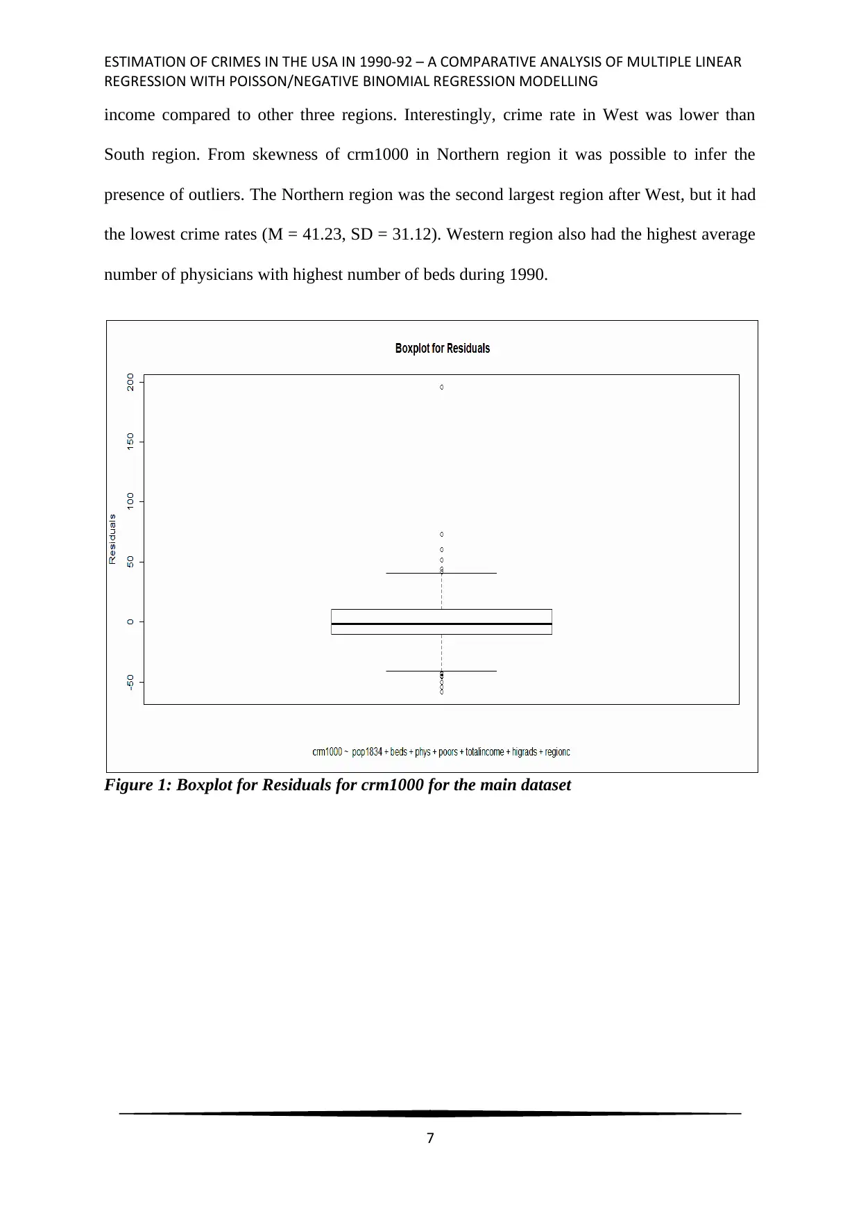
were not distributed normally. Boxplot in Figure 1 affirmed that the data was affected by
presence of outliers, which also adversely affected the multiple regression models. The
sample size was 440, and applying Central Limit theorem the normality was assumed. Table
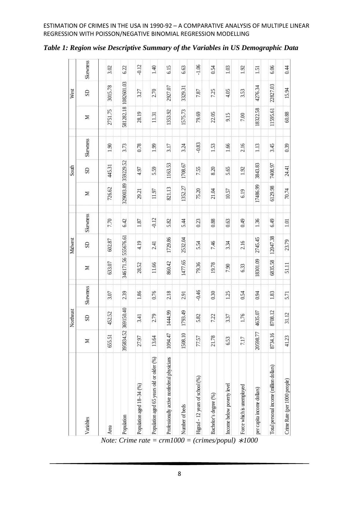
1 presents the detailed descriptive summary of the continuous variables. The region wise
details revealed that West region of the USA was greater in geographical area and total
6
REGRESSION WITH POISSON/NEGATIVE BINOMIAL REGRESSION MODELLING
negative Binomial Regression has been used as it has the same average structure as the
Poisson regression and region as an additional parameter was applied to model the over-
dispersion in Poisson regression model (Osgood, 2000).
The data set of the research was the U.S. county demographic information on 1990-
92. The data set was partitioned in 80:20 ratios for training and testing datasets. The final
linear regression model was checked against the test dataset for appropriate predicting power
of the model.
Descriptive Summary
Crime per thousand people (crm1000) was calculated as crm1000 = (crimes/popul)
∗1000. The average crime rate (crm1000) was 57.29 (SD = 27.33) per thousand people,
considering all regions together. Region wise scrutiny revealed that average crime rate was
41.23 (SD = 31.12) in Northeast, 51.23 (SD = 23.79) in Midwest, 70.74 (SD = 24.41) in
South, and 60.88 (SD = 15.94) in West USA. The Shapiro-Wilk test was used to check for
the normality of the response variable. The test result (W = 0.9, p < 0.05) indicated that
crm1000 was did not follow a normal distribution. Multiple linear regression for crm1000 on
“pop1834”, “phys”, “beds”, “poors”, “totalincome”, “higrads”, and “region”. The residuals
were found be highly right skewed (S = 2.15). Shapiro-Wilk test was conducted to confirm
the pattern of the residuals, and the test statistic (W = 0.88, p < 0.05) revealed that residuals
were not distributed normally. Boxplot in Figure 1 affirmed that the data was affected by
presence of outliers, which also adversely affected the multiple regression models. The
sample size was 440, and applying Central Limit theorem the normality was assumed. Table
1 presents the detailed descriptive summary of the continuous variables. The region wise
details revealed that West region of the USA was greater in geographical area and total
6
⊘ This is a preview!⊘
Do you want full access?
Subscribe today to unlock all pages.
Trusted by 1+ million students worldwide
ESTIMATION OF CRIMES IN THE USA IN 1990-92 – A COMPARATIVE ANALYSIS OF MULTIPLE LINEAR
REGRESSION WITH POISSON/NEGATIVE BINOMIAL REGRESSION MODELLING
income compared to other three regions. Interestingly, crime rate in West was lower than
South region. From skewness of crm1000 in Northern region it was possible to infer the
presence of outliers. The Northern region was the second largest region after West, but it had
the lowest crime rates (M = 41.23, SD = 31.12). Western region also had the highest average
number of physicians with highest number of beds during 1990.
Figure 1: Boxplot for Residuals for crm1000 for the main dataset
7
Paraphrase This Document
Need a fresh take? Get an instant paraphrase of this document with our AI Paraphraser
ESTIMATION OF CRIMES IN THE USA IN 1990-92 – A COMPARATIVE ANALYSIS OF MULTIPLE LINEAR
REGRESSION WITH POISSON/NEGATIVE BINOMIAL REGRESSION MODELLING
Table 1: Region wise Descriptive Summary of the Variables in US Demographic Data
Note: Crime rate = crm1000 = (crimes/popul)
∗1000
8
Variables M SD Skewness M SD Skewness M SD Skewness M SD Skewness
Area 655.51 452.52 3.07 633.07 602.87 7.70 726.62 445.31 1.90 2751.75 3015.78 3.02
Population 395834.52 369150.40 2.39 346171.56 555676.61 6.42 329003.89 359229.52 3.73 581282.18 1082601.03 6.22
Population aged 18–34 (%) 27.97 3.41 1.86 28.52 4.19 1.87 29.21 4.97 0.78 28.19 3.27 -0.12
Population aged 65 years old or older (%) 13.64 2.79 0.76 11.66 2.41 -0.12 11.97 5.59 1.99 11.31 2.70 1.40
Professionally active nonfederal physicians 1094.47 1444.99 2.18 860.42 1729.86 5.82 821.13 1163.53 3.17 1353.92 2927.07 6.15
Number of beds 1508.10 1793.49 2.91 1477.65 2532.04 5.44 1352.27 1708.67 3.24 1575.73 3329.31 6.63
Higrad - 12 years of school (%) 77.57 5.82 -0.46 79.36 5.54 0.23 75.20 7.55 -0.83 79.69 7.87 -1.06
Bachelor’s degree (%) 21.78 7.22 0.30 19.78 7.46 0.88 21.04 8.20 1.53 22.05 7.25 0.54
Income below poverty level 6.53 3.37 1.25 7.90 3.34 0.63 10.57 5.65 1.66 9.15 4.05 1.03
Force which is unemployed 7.17 1.76 0.54 6.33 2.16 0.49 6.19 1.92 2.16 7.00 3.53 1.92
per capita income dollars) 20598.77 4635.07 0.94 18301.09 2745.45 1.36 17486.99 3843.83 1.13 18322.58 4276.34 1.51
Total personal income (million dollars) 8734.16 8708.12 1.83 6835.58 12047.38 6.49 6129.98 7408.97 3.45 11595.61 22827.03 6.06
Crime Rate (per 1000 people) 41.23 31.12 5.71 51.11 23.79 1.01 70.74 24.41 0.39 60.88 15.94 0.44
Northeast Midwest South West
ESTIMATION OF CRIMES IN THE USA IN 1990-92 – A COMPARATIVE ANALYSIS OF MULTIPLE LINEAR
REGRESSION WITH POISSON/NEGATIVE BINOMIAL REGRESSION MODELLING
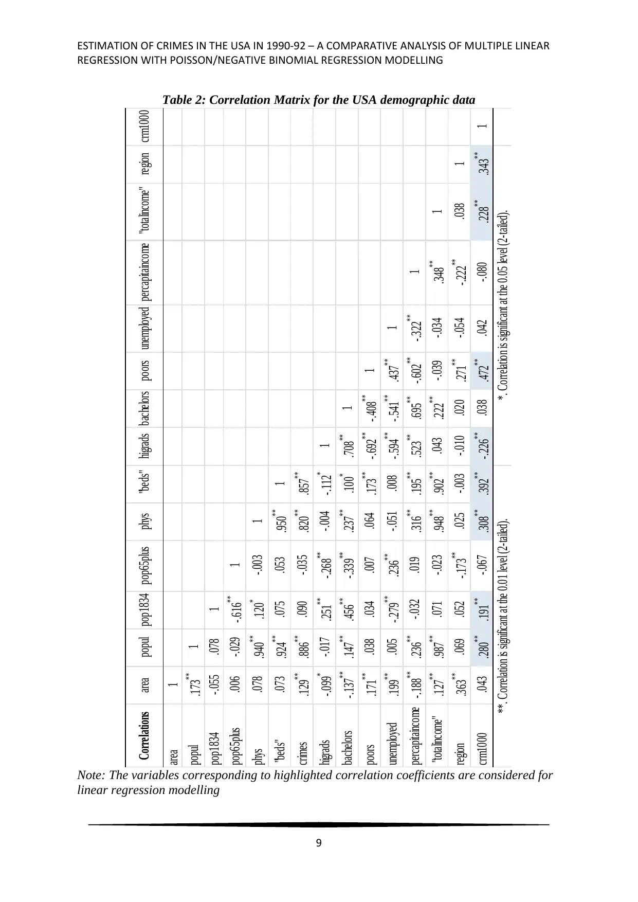
Table 2: Correlation Matrix for the USA demographic data
Note: The variables corresponding to highlighted correlation coefficients are considered for
linear regression modelling
9
Correlations area popul pop1834 pop65plus phys "beds" higrads bachelors poors unemployed percapitaincome "totalincome" region crm1000
area 1
popul .173 ** 1
pop1834 -.055 .078 1
pop65plus .006 -.029 -.616
** 1
phys .078 .940
** .120
* -.003 1
"beds" .073 .924
** .075 .053 .950 ** 1
crimes .129 ** .886
** .090 -.035 .820 ** .857 **
higrads -.099 * -.017 .251 ** -.268
** -.004 -.112
* 1
bachelors -.137 ** .147
** .456 ** -.339
** .237 ** .100 * .708 ** 1
poors .171 ** .038 .034 .007 .064 .173 ** -.692 ** -.408 ** 1
unemployed .199 ** .005 -.279
** .236 ** -.051 .008 -.594 ** -.541 ** .437 ** 1
percapitaincome -.188 ** .236
** -.032 .019 .316 ** .195 ** .523 ** .695 ** -.602 ** -.322 ** 1
"totalincome" .127 ** .987
** .071 -.023 .948 ** .902 ** .043 .222 ** -.039 -.034 .348 ** 1
region .363 ** .069 .052 -.173
** .025 -.003 -.010 .020 .271 ** -.054 -.222 ** .038 1
crm1000 .043 .280
** .191 ** -.067 .308 ** .392 ** -.226 ** .038 .472 ** .042 -.080 .228
** .343
** 1
**. Correlation is significant at the 0.01 level (2-tailed). *. Correlation is significant at the 0.05 level (2-tailed).
REGRESSION WITH POISSON/NEGATIVE BINOMIAL REGRESSION MODELLING
Table 2: Correlation Matrix for the USA demographic data
Note: The variables corresponding to highlighted correlation coefficients are considered for
linear regression modelling
9
Correlations area popul pop1834 pop65plus phys "beds" higrads bachelors poors unemployed percapitaincome "totalincome" region crm1000
area 1
popul .173 ** 1
pop1834 -.055 .078 1
pop65plus .006 -.029 -.616
** 1
phys .078 .940
** .120
* -.003 1
"beds" .073 .924
** .075 .053 .950 ** 1
crimes .129 ** .886
** .090 -.035 .820 ** .857 **
higrads -.099 * -.017 .251 ** -.268
** -.004 -.112
* 1
bachelors -.137 ** .147
** .456 ** -.339
** .237 ** .100 * .708 ** 1
poors .171 ** .038 .034 .007 .064 .173 ** -.692 ** -.408 ** 1
unemployed .199 ** .005 -.279
** .236 ** -.051 .008 -.594 ** -.541 ** .437 ** 1
percapitaincome -.188 ** .236
** -.032 .019 .316 ** .195 ** .523 ** .695 ** -.602 ** -.322 ** 1
"totalincome" .127 ** .987
** .071 -.023 .948 ** .902 ** .043 .222 ** -.039 -.034 .348 ** 1
region .363 ** .069 .052 -.173
** .025 -.003 -.010 .020 .271 ** -.054 -.222 ** .038 1
crm1000 .043 .280
** .191 ** -.067 .308 ** .392 ** -.226 ** .038 .472 ** .042 -.080 .228
** .343
** 1
**. Correlation is significant at the 0.01 level (2-tailed). *. Correlation is significant at the 0.05 level (2-tailed).
⊘ This is a preview!⊘
Do you want full access?
Subscribe today to unlock all pages.
Trusted by 1+ million students worldwide
ESTIMATION OF CRIMES IN THE USA IN 1990-92 – A COMPARATIVE ANALYSIS OF MULTIPLE LINEAR
REGRESSION WITH POISSON/NEGATIVE BINOMIAL REGRESSION MODELLING
Multiple Regression Analysis
Outlier Detection
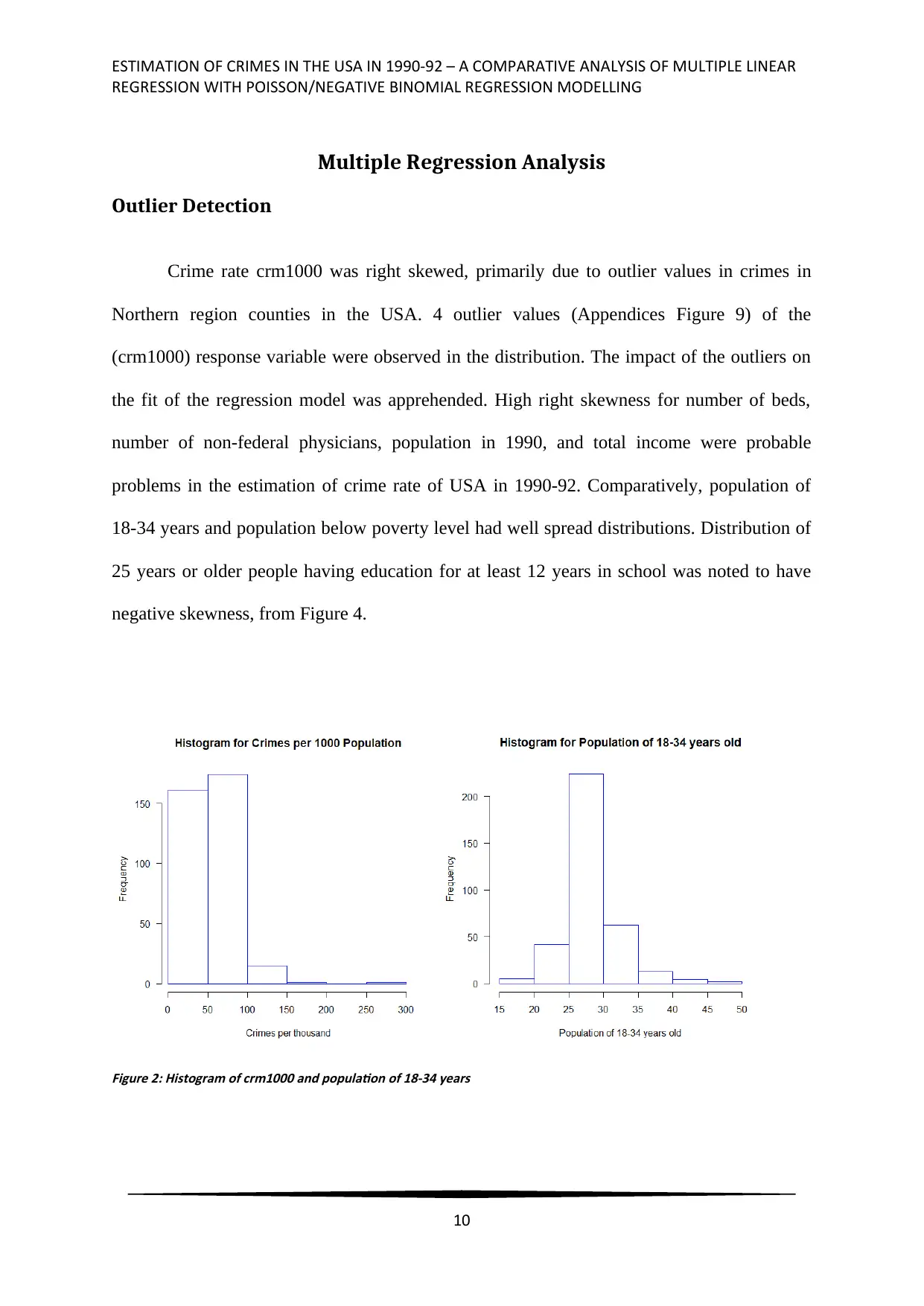
Crime rate crm1000 was right skewed, primarily due to outlier values in crimes in
Northern region counties in the USA. 4 outlier values (Appendices Figure 9) of the
(crm1000) response variable were observed in the distribution. The impact of the outliers on
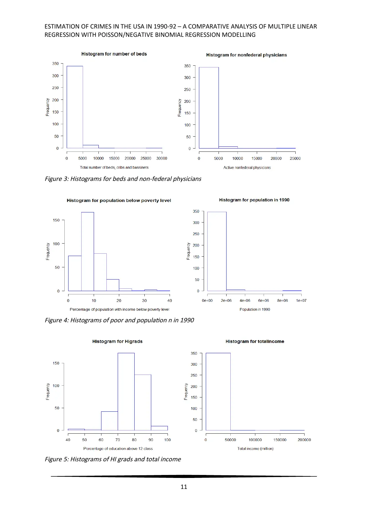
the fit of the regression model was apprehended. High right skewness for number of beds,
number of non-federal physicians, population in 1990, and total income were probable
problems in the estimation of crime rate of USA in 1990-92. Comparatively, population of
18-34 years and population below poverty level had well spread distributions. Distribution of
25 years or older people having education for at least 12 years in school was noted to have
negative skewness, from Figure 4.
Figure 2: Histogram of crm1000 and population of 18-34 years
10
REGRESSION WITH POISSON/NEGATIVE BINOMIAL REGRESSION MODELLING
Multiple Regression Analysis
Outlier Detection
Crime rate crm1000 was right skewed, primarily due to outlier values in crimes in
Northern region counties in the USA. 4 outlier values (Appendices Figure 9) of the
(crm1000) response variable were observed in the distribution. The impact of the outliers on
the fit of the regression model was apprehended. High right skewness for number of beds,
number of non-federal physicians, population in 1990, and total income were probable
problems in the estimation of crime rate of USA in 1990-92. Comparatively, population of
18-34 years and population below poverty level had well spread distributions. Distribution of
25 years or older people having education for at least 12 years in school was noted to have
negative skewness, from Figure 4.
Figure 2: Histogram of crm1000 and population of 18-34 years
10
Paraphrase This Document
Need a fresh take? Get an instant paraphrase of this document with our AI Paraphraser
ESTIMATION OF CRIMES IN THE USA IN 1990-92 – A COMPARATIVE ANALYSIS OF MULTIPLE LINEAR
REGRESSION WITH POISSON/NEGATIVE BINOMIAL REGRESSION MODELLING
Figure 3: Histograms for beds and non-federal physicians
Figure 4: Histograms of poor and population n in 1990
Figure 5: Histograms of HI grads and total income
11
REGRESSION WITH POISSON/NEGATIVE BINOMIAL REGRESSION MODELLING
Figure 3: Histograms for beds and non-federal physicians
Figure 4: Histograms of poor and population n in 1990
Figure 5: Histograms of HI grads and total income
11
ESTIMATION OF CRIMES IN THE USA IN 1990-92 – A COMPARATIVE ANALYSIS OF MULTIPLE LINEAR
REGRESSION WITH POISSON/NEGATIVE BINOMIAL REGRESSION MODELLING
Correlation Analysis
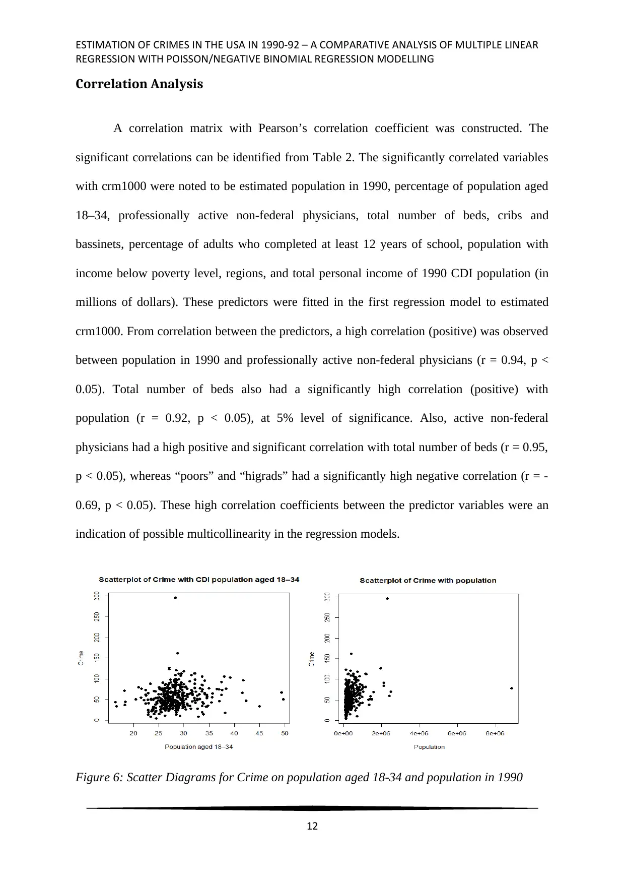
A correlation matrix with Pearson’s correlation coefficient was constructed. The
significant correlations can be identified from Table 2. The significantly correlated variables
with crm1000 were noted to be estimated population in 1990, percentage of population aged
18–34, professionally active non-federal physicians, total number of beds, cribs and
bassinets, percentage of adults who completed at least 12 years of school, population with
income below poverty level, regions, and total personal income of 1990 CDI population (in
millions of dollars). These predictors were fitted in the first regression model to estimated
crm1000. From correlation between the predictors, a high correlation (positive) was observed
between population in 1990 and professionally active non-federal physicians (r = 0.94, p <
0.05). Total number of beds also had a significantly high correlation (positive) with
population (r = 0.92, p < 0.05), at 5% level of significance. Also, active non-federal
physicians had a high positive and significant correlation with total number of beds (r = 0.95,
p < 0.05), whereas “poors” and “higrads” had a significantly high negative correlation (r = -
0.69, p < 0.05). These high correlation coefficients between the predictor variables were an
indication of possible multicollinearity in the regression models.
Figure 6: Scatter Diagrams for Crime on population aged 18-34 and population in 1990
12
REGRESSION WITH POISSON/NEGATIVE BINOMIAL REGRESSION MODELLING
Correlation Analysis
A correlation matrix with Pearson’s correlation coefficient was constructed. The
significant correlations can be identified from Table 2. The significantly correlated variables
with crm1000 were noted to be estimated population in 1990, percentage of population aged
18–34, professionally active non-federal physicians, total number of beds, cribs and
bassinets, percentage of adults who completed at least 12 years of school, population with
income below poverty level, regions, and total personal income of 1990 CDI population (in
millions of dollars). These predictors were fitted in the first regression model to estimated
crm1000. From correlation between the predictors, a high correlation (positive) was observed
between population in 1990 and professionally active non-federal physicians (r = 0.94, p <
0.05). Total number of beds also had a significantly high correlation (positive) with
population (r = 0.92, p < 0.05), at 5% level of significance. Also, active non-federal
physicians had a high positive and significant correlation with total number of beds (r = 0.95,
p < 0.05), whereas “poors” and “higrads” had a significantly high negative correlation (r = -
0.69, p < 0.05). These high correlation coefficients between the predictor variables were an
indication of possible multicollinearity in the regression models.
Figure 6: Scatter Diagrams for Crime on population aged 18-34 and population in 1990
12
⊘ This is a preview!⊘
Do you want full access?
Subscribe today to unlock all pages.
Trusted by 1+ million students worldwide
1 out of 31
Your All-in-One AI-Powered Toolkit for Academic Success.
+13062052269
info@desklib.com
Available 24*7 on WhatsApp / Email
![[object Object]](/_next/static/media/star-bottom.7253800d.svg)
Unlock your academic potential
Copyright © 2020–2026 A2Z Services. All Rights Reserved. Developed and managed by ZUCOL.