Regression Analysis on Vehicle Sales Price Influencing Factors

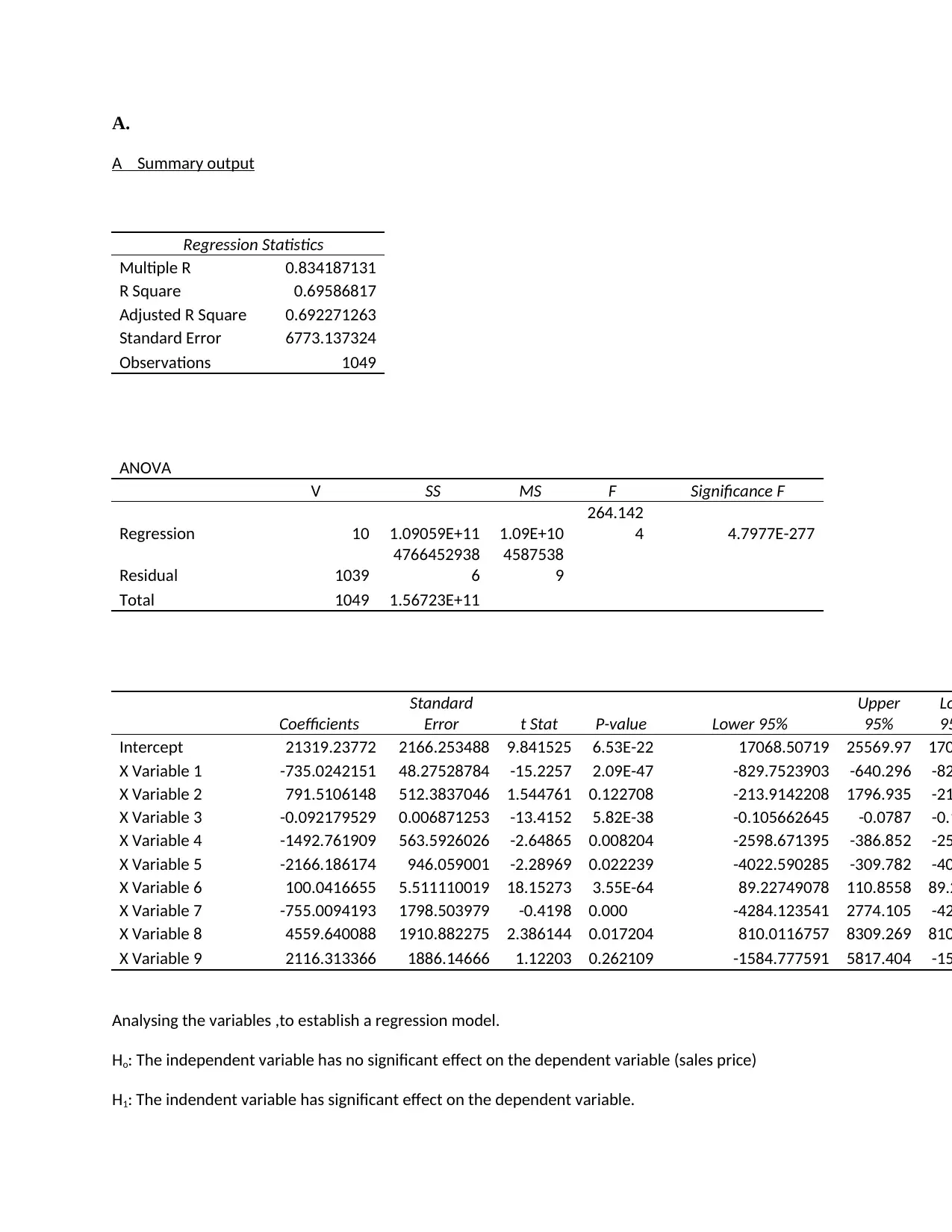
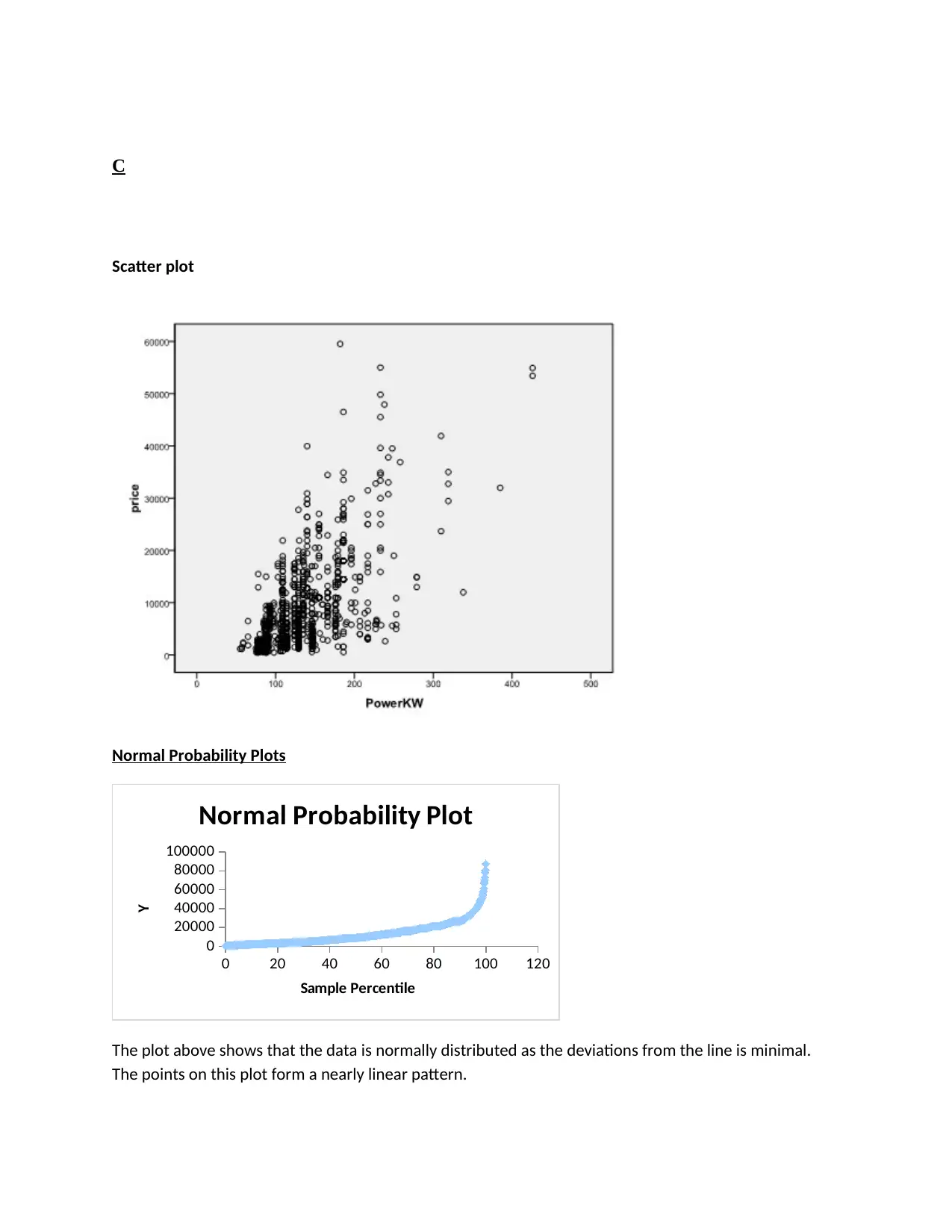
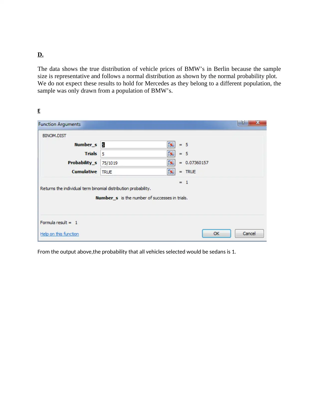
The assignment presents a summary output of a regression model aimed at predicting used vehicle sales prices based on various independent variables. Key statistical indicators such as Multiple R (0.834187131), R Square (0.69586817), Adjusted R Square (0.692271263), and an ANOVA table with significant F-values demonstrate the overall effectiveness of the regression model. Hypotheses testing reveals that variables X1, X3, X4, X5, X6, X7, and X8 are statistically significant at a 5% significance level as their p-values are less than 0.05. Conversely, variables X2 and X9 do not significantly impact sales prices, leading to their exclusion from the final model. The refined regression equation is Y = 21319.23772 - 735.0242151X1 - 0.092179529X3 - 1492.761909X4 - 2166.186174X5 + 100.0416655X6 - 755.0094193X7 + 4559.640088X8, where Y represents the sales price and X1 to X9 are specific vehicle attributes such as age, kilometers driven, fuel type, power in KW, etc. Additional analysis includes a scatter plot indicating normal distribution based on minimal deviations from a reference line. The study concludes that while the results are representative of BMWs in Berlin, they may not generalize to other brands like Mercedes due to differing population characteristics.

A.
A Summary output
Regression Statistics
Multiple R 0.834187131
R Square 0.69586817
Adjusted R Square 0.692271263
Standard Error 6773.137324
Observations 1049
ANOVA
V SS MS F Significance F
Regression 10 1.09059E+11 1.09E+10
264.142
4 4.7977E-277
Residual 1039
4766452938
6
4587538
9
Total 1049 1.56723E+11
Coefficients
Standard
Error t Stat P-value Lower 95%
Upper
95%
Lo
95
Intercept 21319.23772 2166.253488 9.841525 6.53E-22 17068.50719 25569.97 170
X Variable 1 -735.0242151 48.27528784 -15.2257 2.09E-47 -829.7523903 -640.296 -82
X Variable 2 791.5106148 512.3837046 1.544761 0.122708 -213.9142208 1796.935 -21
X Variable 3 -0.092179529 0.006871253 -13.4152 5.82E-38 -0.105662645 -0.0787 -0.1
X Variable 4 -1492.761909 563.5926026 -2.64865 0.008204 -2598.671395 -386.852 -25
X Variable 5 -2166.186174 946.059001 -2.28969 0.022239 -4022.590285 -309.782 -40
X Variable 6 100.0416655 5.511110019 18.15273 3.55E-64 89.22749078 110.8558 89.2
X Variable 7 -755.0094193 1798.503979 -0.4198 0.000 -4284.123541 2774.105 -42
X Variable 8 4559.640088 1910.882275 2.386144 0.017204 810.0116757 8309.269 810
X Variable 9 2116.313366 1886.14666 1.12203 0.262109 -1584.777591 5817.404 -15
Analysing the variables ,to establish a regression model.
Ho: The independent variable has no significant effect on the dependent variable (sales price)
H1: The indendent variable has significant effect on the dependent variable.

We compare the p-values at 5% level of significance for the independent variables.
Variables 1, 3 ,4,5 ,6,7,8 have their p-values being less than 0.05 thus they are will be part of our model
as independent variables. The variables 2 and 9 have their p-values being greater than 0.05 hence we
fail to reject the null hypothesis and conclude that they are insignificant in explaining the sales price.
Model becomes:
Y=21319.23772-735.0242151X1-0.092179529X3-1492.761909X4-2166.186174X5+100.0416655X6-
755.0094193X7+4559.640088X8
Where:
Y= Sales price
X1:Age
X2:automatic
X3:kilo metres
X4:petrol
X5:damage
X6: power KW
X7:Sedan
X8:convertible
X9:coupe
Other factors that might have influenced sales price of the used vehicles include the country of origin.
B
It is appropriate to predict sales price under the given conditions
Y= 21319.23772-735.0242151(5)-0.092179529(75000)-1492.761909-100.0416655(110)-
755.0094193=4,828.5302

C
Scatter plot
Normal Probability Plots
0 20 40 60 80 100 120
0
20000
40000
60000
80000
100000
Normal Probability Plot
Sample Percentile
Y
The plot above shows that the data is normally distributed as the deviations from the line is minimal.
The points on this plot form a nearly linear pattern.

D.
The data shows the true distribution of vehicle prices of BMW’s in Berlin because the sample
size is representative and follows a normal distribution as shown by the normal probability plot.
We do not expect these results to hold for Mercedes as they belong to a different population, the
sample was only drawn from a population of BMW’s.
E
From the output above,the probability that all vehicles selected would be sedans is 1.

The probability that of the selected vehicles, none would be a sedan is 0.682321493 as shown by the
above output.
A bar chart showing the probability distribution of the number of vehicles that are sedans
1
2
3
4
5
6
0 0.2 0.4 0.6 0.8 1 1.2
Series1

References
Abrahams, S.T. and Keve, E.T., 1971. Normal probability plot analysis of error in measured and derived
quantities and standard deviations. Acta Crystallographica Section A: Crystal Physics, Diffraction,
Theoretical and General Crystallography, 27(2), pp.157-165.
Mosteller, F. and Tukey, J.W., 1977. Data analysis and regression: a second course in statistics. Addison-
Wesley Series in Behavioral Science: Quantitative Methods.
Skellam, J.G., 1948. A probability distribution derived from the binomial distribution by regarding the
probability of success as variable between the sets of trials. Journal of the Royal Statistical Society. Series
B (Methodological), 10(2), pp.257-261
Ciuiu, D., 2010. Informational Criteria for the Homoscedasticity of Errors. Romanian Journal of Economic
Forecasting, 13(2), pp.231-244.