ECMT1010 Statistics Assignment: Wage Regression and Hypothesis

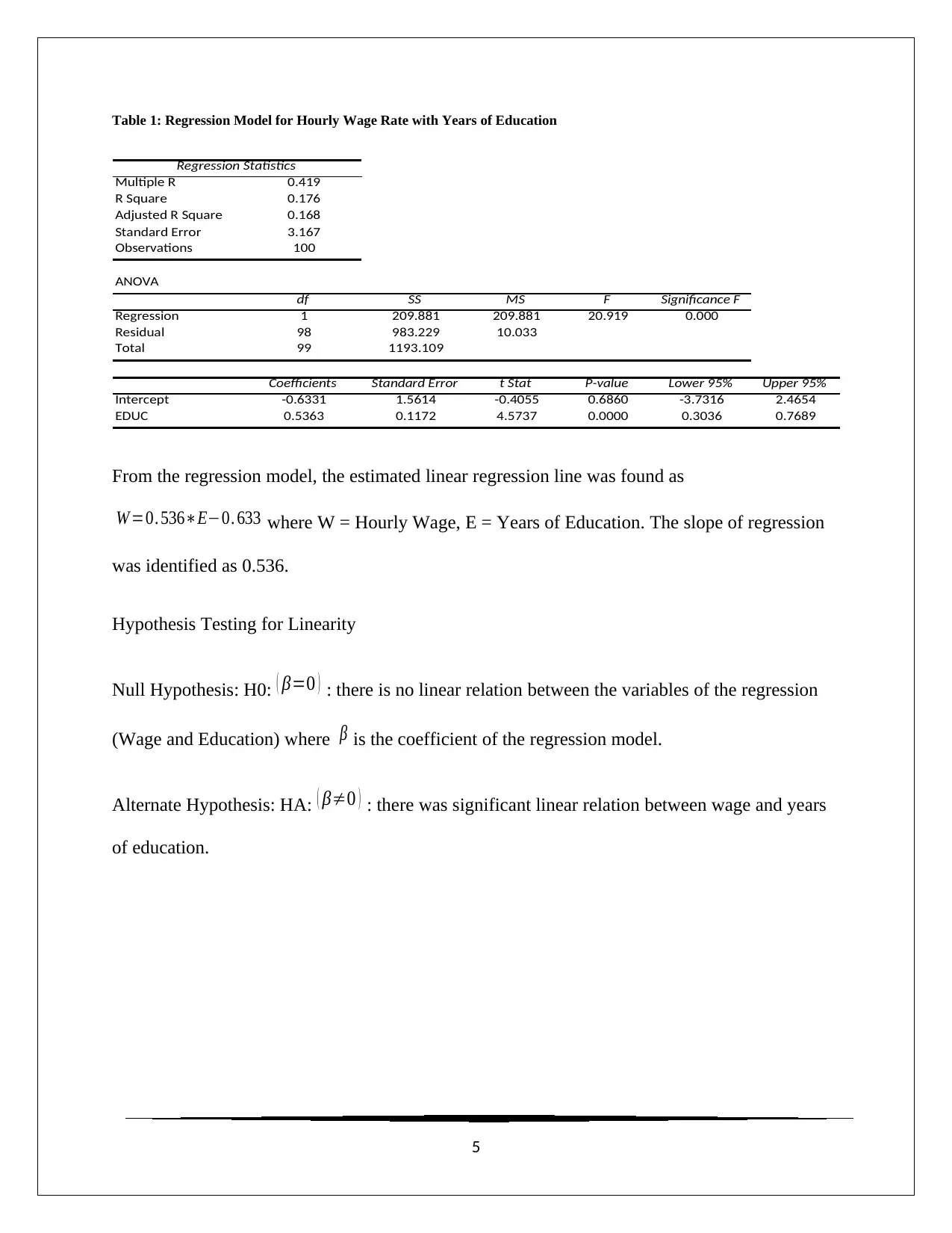
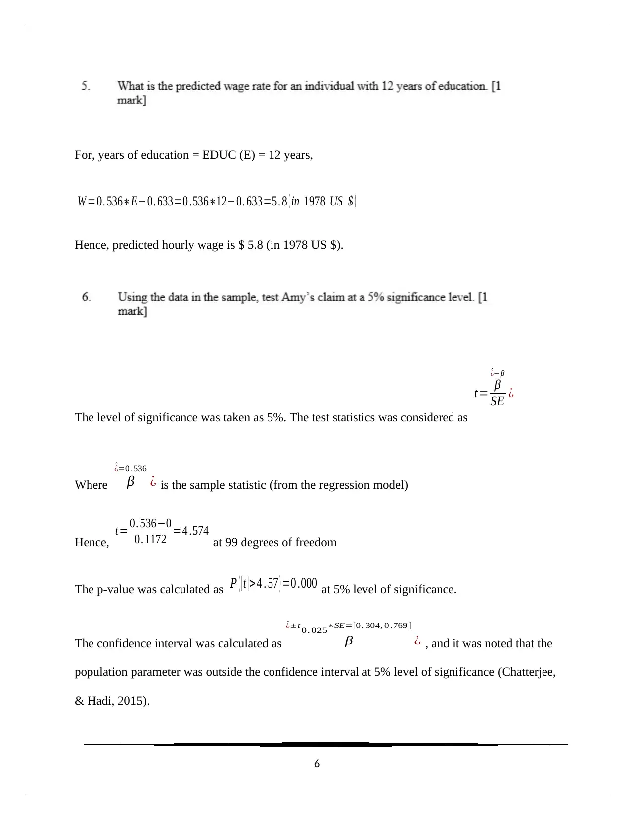
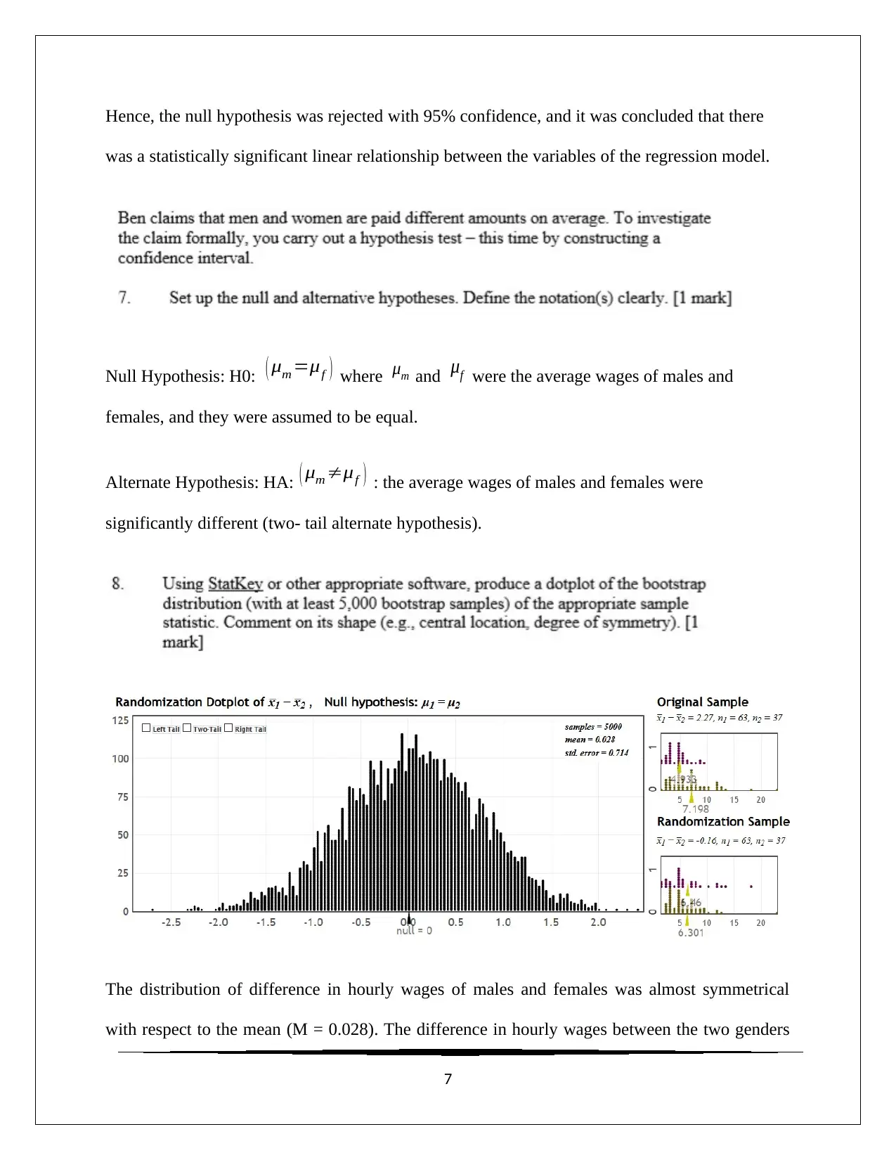
This ECMT1010 statistics assignment from the University of Sydney explores the relationship between hourly wages, education levels, and gender using data from 1978. The analysis includes descriptive statistics, histograms, scatter plots, and regression modeling to determine the impact of education on wages. Hypothesis testing is conducted to assess the significance of the linear relationship between wage and education, as well as to compare average wages between males and females. The findings suggest a positive correlation between education and hourly wage and indicate statistically significant differences in pay between genders, possibly reflecting gender discrimination prevalent at the time. The assignment references statistical methods and tools, concluding with insights into wage disparities and their potential causes, all of which can be further explored with similar resources available on Desklib.

Statistics Assignment
ECMT1010
1

Figure 1: Histogram for Wages of Males in Hour
Figure 2: Histogram for Wages of Females in Hour
2

Distribution of hourly wage rate of males was found to be positively skewed (S = 1.64) with
Median of hourly wage rate at 6.25 (in 1978 US $). The dispersion (inter-quartile range) of
hourly wage rates was found to be 3.64 (in 1978 US $). Distribution of hourly wage rate of
females was found to be almost normal with slight positive skewness (S = 0.67) with median of
hourly wage rate at 5.0 (in 1978 US $). The dispersion (inter-quartile range) of hourly wage rates
was found to be 2.41 (in 1978 US $). Most of the males were found to get hourly wages towards
the first quartile of the range of their hourly wages, indicating presence of outlier hourly wage
for few males. Females’ hourly wages were almost normally distributed in the range of their
hourly wages, indicating symmetric division of hourly wages for females.
The average hourly wage rate of 7.20 (in 1978 US $)
The standard deviation of hourly wage rates was found to be 3.87 (in 1978 US $)
Average hourly wage rate of 4.93 (in 1978 US $)
The standard deviation of hourly wage rates was found to be 2.01 (in 1978 US $).
3

Figure 3: Scatter-plot of Hourly Wage with respect to Year of Education
Correlation between hourly wage and year of education was (r= 0.419, p < 0.05) positive and
significant. Hourly wage was found to positively and linearly depend on year of education of the
employee.
4

Table 1: Regression Model for Hourly Wage Rate with Years of Education
Regression Statistics
Multiple R 0.419
R Square 0.176
Adjusted R Square 0.168
Standard Error 3.167
Observations 100
ANOVA
df SS MS F Significance F
Regression 1 209.881 209.881 20.919 0.000
Residual 98 983.229 10.033
Total 99 1193.109
Coefficients Standard Error t Stat P-value Lower 95% Upper 95%
Intercept -0.6331 1.5614 -0.4055 0.6860 -3.7316 2.4654
EDUC 0.5363 0.1172 4.5737 0.0000 0.3036 0.7689
From the regression model, the estimated linear regression line was found as
W =0. 536∗E−0. 633 where W = Hourly Wage, E = Years of Education. The slope of regression
was identified as 0.536.
Hypothesis Testing for Linearity
Null Hypothesis: H0: ( β=0 ) : there is no linear relation between the variables of the regression
(Wage and Education) where β is the coefficient of the regression model.
Alternate Hypothesis: HA: ( β≠0 ) : there was significant linear relation between wage and years
of education.
5

For, years of education = EDUC (E) = 12 years,
W =0. 536∗E−0. 633=0 .536∗12−0. 633=5. 8 ( in 1978 US $ )
Hence, predicted hourly wage is $ 5.8 (in 1978 US $).
The level of significance was taken as 5%. The test statistics was considered as
t= β
^¿− β
SE ¿
Where β
^¿=0 .536
¿ is the sample statistic (from the regression model)
Hence, t = 0. 536−0
0. 1172 =4 .574 at 99 degrees of freedom
The p-value was calculated as P (|t|>4 . 57 ) =0 .000 at 5% level of significance.
The confidence interval was calculated as β
^¿±t 0. 025∗SE=[0 . 304, 0 .769 ]
¿ , and it was noted that the
population parameter was outside the confidence interval at 5% level of significance (Chatterjee,
& Hadi, 2015).
6

Hence, the null hypothesis was rejected with 95% confidence, and it was concluded that there
was a statistically significant linear relationship between the variables of the regression model.
Null Hypothesis: H0: ( μm =μf ) where μm and μf were the average wages of males and
females, and they were assumed to be equal.
Alternate Hypothesis: HA: ( μm ≠μf ) : the average wages of males and females were
significantly different (two- tail alternate hypothesis).
The distribution of difference in hourly wages of males and females was almost symmetrical
with respect to the mean (M = 0.028). The difference in hourly wages between the two genders
7

was distributed symmetrically about zero, which implied that average hourly wages of the two
genders were almost equal in the population data.
From the two methods of 95% confidence interval, it was identified that the average estimated
difference in hourly wages between the two genders was somewhere between the specified
intervals, which does not contain the hypothesized mean difference ( μ1−μ2=0 ). Hence, with
8

95% confidence it was possible to state that Ben’s claim was statistically significant (Morgan,
Lock, Lock, Lock, & Lock, 2014).
From the statistical analysis it could be inferred that men and women were paid differently. The
gender discrimination could be a possible reason for the difference in their rates of hourly wages
in 1978, probably due to the social condition at that time.
References
Chatterjee, S., & Hadi, A. S. (2015). Regression analysis by example. John Wiley & Sons.
Morgan, K. L., Lock, R. H., Lock, P. F., Lock, E. F., & Lock, D. F. (2014, July). StatKey: Online
tools for bootstrap intervals and randomization tests. In Sustainability in statistics
education. Proceedings of the 9th International Conference on Teaching Statistics,
ICOTS9.
9