Web Analytics at Quality Alloys Inc: BI and Data Visualization Report
VerifiedAdded on 2023/03/31
|19
|3637
|269
Report
AI Summary
This report analyzes the web analytics data of Quality Alloys, Inc. (QA), a distributor of alloys, focusing on website traffic, revenue, profit, and pounds sold over time. The analysis covers an initial period, a pre-promotion period, a promotion period, and a post-promotion period. Descriptive statistics, including mean, median, standard deviation, minimum, and maximum values, are calculated for each period to identify trends and relationships between variables. The report finds that website visits were highest between February and April, but sales did not significantly increase, suggesting a need for alternative marketing strategies and enabling online ordering. A positive correlation between revenue and pounds sold is also identified.

Statistics
Business intelligence and data visualization
Student name:
Tutor name:
1 | P a g e
Business intelligence and data visualization
Student name:
Tutor name:
1 | P a g e
Paraphrase This Document
Need a fresh take? Get an instant paraphrase of this document with our AI Paraphraser
Statistics
Executive summary
Similar to some other enterprise QA company in its operations faces competition from different
corporations which might be producing similar products. So as to grow its sales through
widening its market, it established an internet site in which customers would learn more about
the organization. Diverse records have been kept about what took place in the internet site over a
time frame. These records were analyzed and presented in form of tables and graphs. The
consequences confirmed that variety of specific visits to the website become excessive between
February and March. However, sales and the wide variety of pounds bought over the period
seemed not to enhance. This become glaring as earnings have been handiest excessive for the
duration of the pre-promotion length and then it decreased. The research recommends to the
management of QA to give you other marketing avenues aside from the website to power
income. They must also allow customers to location orders thru the website as the research has
installed that there are many individuals who visit the website.
2 | P a g e
Statistics
QUESTION ONE
Descriptive statistics
Unique visits to the QA website per week
May 25 - May 31
Jun 15 - Jun 21
Jul 6 - Jul 12
Jul 27 - Aug 2
Aug 17 - Aug 23
Sep 7 - Sep 13
Sep 28 - Oct 4
Oct 19 - Oct 25
Nov 9 - Nov 15
Nov 30 - Dec 6
Dec 21 - Dec 27
Jan 11 - Jan 17
Feb 1 - Feb 7
Feb 22 - Feb 28
Mar 15 - Mar 21
Apr 5 - Apr 11
Apr 26 - May 2
May 17 - May 23
Jun 7 - Jun 13
Jun 28 - Jul 4
Jul 19 - Jul 25
Aug 9 - Aug 15
0
500
1,000
1,500
2,000
2,500
3,000
3,500
4,000
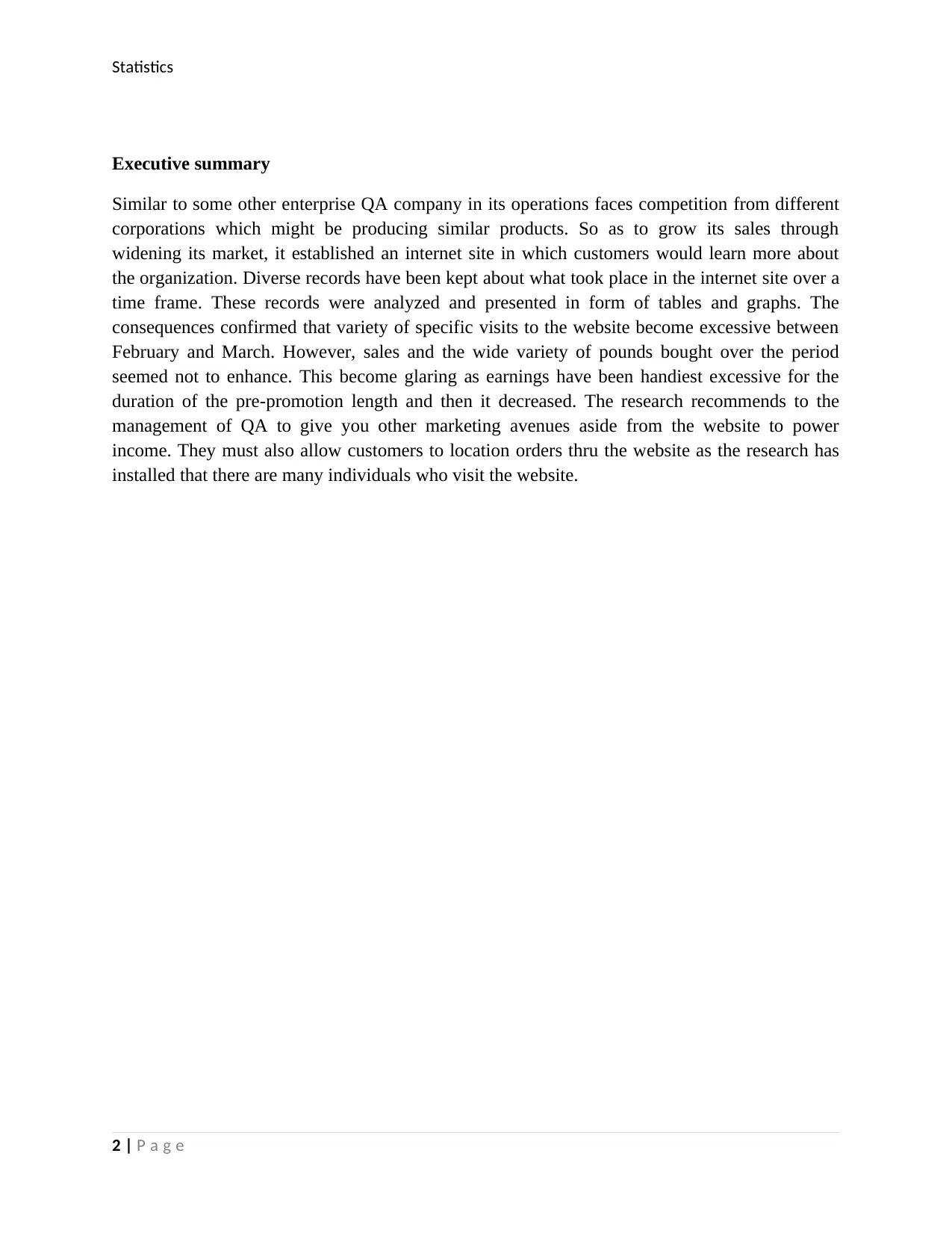
Figure 1. Unique Visits to the QA website
per week
Figure 1
The bar graph above shows the frequency of unique visits to QA website per week from May
25th 2008 to August 15th 2009. It can be observed that the number of unique visits to the website
was high between February 1st and April 11th. This is after a decline was observed from May 25th
to around December 21st 2008. To add on, another decline in the number of visits to the website
starts from February 22nd 2009 to 15th August 2009.
Revenue over time per week
3 | P a g e
QUESTION ONE
Descriptive statistics
Unique visits to the QA website per week
May 25 - May 31
Jun 15 - Jun 21
Jul 6 - Jul 12
Jul 27 - Aug 2
Aug 17 - Aug 23
Sep 7 - Sep 13
Sep 28 - Oct 4
Oct 19 - Oct 25
Nov 9 - Nov 15
Nov 30 - Dec 6
Dec 21 - Dec 27
Jan 11 - Jan 17
Feb 1 - Feb 7
Feb 22 - Feb 28
Mar 15 - Mar 21
Apr 5 - Apr 11
Apr 26 - May 2
May 17 - May 23
Jun 7 - Jun 13
Jun 28 - Jul 4
Jul 19 - Jul 25
Aug 9 - Aug 15
0
500
1,000
1,500
2,000
2,500
3,000
3,500
4,000
Figure 1. Unique Visits to the QA website
per week
Figure 1
The bar graph above shows the frequency of unique visits to QA website per week from May
25th 2008 to August 15th 2009. It can be observed that the number of unique visits to the website
was high between February 1st and April 11th. This is after a decline was observed from May 25th
to around December 21st 2008. To add on, another decline in the number of visits to the website
starts from February 22nd 2009 to 15th August 2009.
Revenue over time per week
3 | P a g e
⊘ This is a preview!⊘
Do you want full access?
Subscribe today to unlock all pages.
Trusted by 1+ million students worldwide
Statistics
May 25 - May 31
Jun 22 - Jun 28
Jul 20 - Jul 26
Aug 17 - Aug 23
Sep 14 - Sep 20
Oct 12 - Oct 18
Nov 9 - Nov 15
Dec 7 - Dec 13
Jan 4 - Jan 10
Feb 1 - Feb 7
Mar 1 - Mar 7
Mar 29 - Apr 4
Apr 26 - May 2
May 24 - May 30
Jun 21 - Jun 27
Jul 19 - Jul 25
Aug 16 - Aug 22
$0
$200,000
$400,000
$600,000
$800,000
$1,000,000
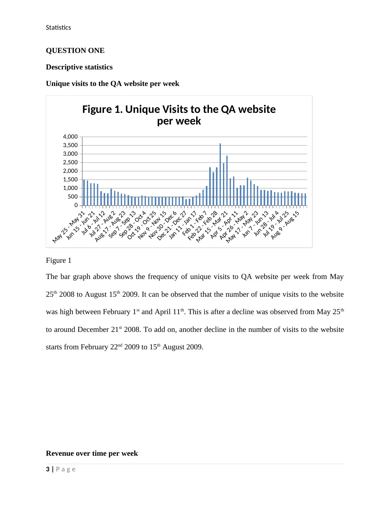
Figure 2. Revenue over time per
week
Figure 2
The figure above is of graph of revenue got by QA per week over a period of time. as can be
observed, no particular pattern can be seen from the frequencies. It can be said that the
frequencies for the revenue per week is relatively uniform throughout the period.
Profit over time per week
May 25 - May 31
Jun 22 - Jun 28
Jul 20 - Jul 26
Aug 17 - Aug 23
Sep 14 - Sep 20
Oct 12 - Oct 18
Nov 9 - Nov 15
Dec 7 - Dec 13
Jan 4 - Jan 10
Feb 1 - Feb 7
Mar 1 - Mar 7
Mar 29 - Apr 4
Apr 26 - May 2
May 24 - May 30
Jun 21 - Jun 27
Jul 19 - Jul 25
Aug 16 - Aug 22
$0
$50,000
$100,000
$150,000
$200,000
$250,000
$300,000
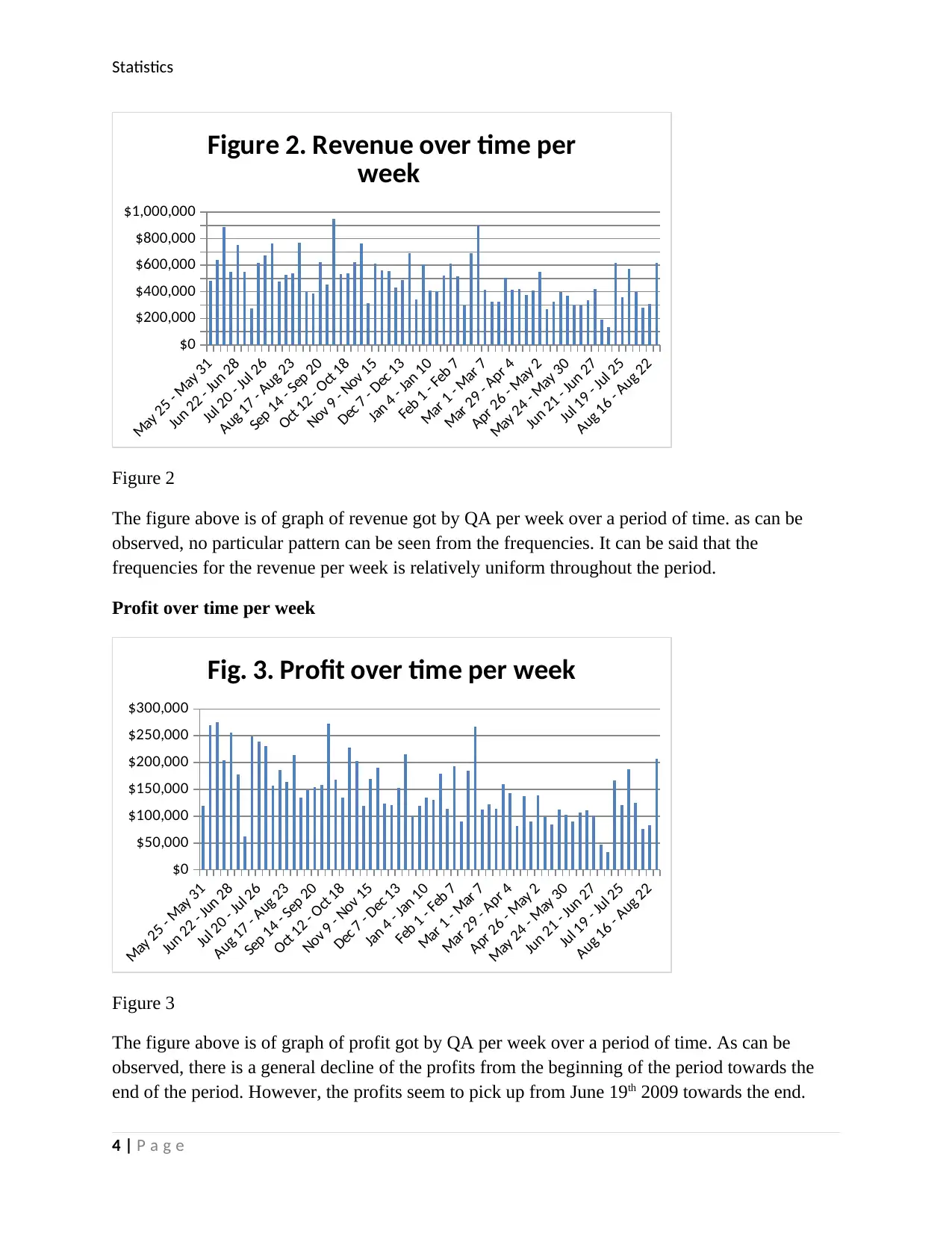
Fig. 3. Profit over time per week
Figure 3
The figure above is of graph of profit got by QA per week over a period of time. As can be
observed, there is a general decline of the profits from the beginning of the period towards the
end of the period. However, the profits seem to pick up from June 19th 2009 towards the end.
4 | P a g e
May 25 - May 31
Jun 22 - Jun 28
Jul 20 - Jul 26
Aug 17 - Aug 23
Sep 14 - Sep 20
Oct 12 - Oct 18
Nov 9 - Nov 15
Dec 7 - Dec 13
Jan 4 - Jan 10
Feb 1 - Feb 7
Mar 1 - Mar 7
Mar 29 - Apr 4
Apr 26 - May 2
May 24 - May 30
Jun 21 - Jun 27
Jul 19 - Jul 25
Aug 16 - Aug 22
$0
$200,000
$400,000
$600,000
$800,000
$1,000,000
Figure 2. Revenue over time per
week
Figure 2
The figure above is of graph of revenue got by QA per week over a period of time. as can be
observed, no particular pattern can be seen from the frequencies. It can be said that the
frequencies for the revenue per week is relatively uniform throughout the period.
Profit over time per week
May 25 - May 31
Jun 22 - Jun 28
Jul 20 - Jul 26
Aug 17 - Aug 23
Sep 14 - Sep 20
Oct 12 - Oct 18
Nov 9 - Nov 15
Dec 7 - Dec 13
Jan 4 - Jan 10
Feb 1 - Feb 7
Mar 1 - Mar 7
Mar 29 - Apr 4
Apr 26 - May 2
May 24 - May 30
Jun 21 - Jun 27
Jul 19 - Jul 25
Aug 16 - Aug 22
$0
$50,000
$100,000
$150,000
$200,000
$250,000
$300,000
Fig. 3. Profit over time per week
Figure 3
The figure above is of graph of profit got by QA per week over a period of time. As can be
observed, there is a general decline of the profits from the beginning of the period towards the
end of the period. However, the profits seem to pick up from June 19th 2009 towards the end.
4 | P a g e
Paraphrase This Document
Need a fresh take? Get an instant paraphrase of this document with our AI Paraphraser
Statistics
Pounds over time per week
May 25 - May 31
Jun 22 - Jun 28
Jul 20 - Jul 26
Aug 17 - Aug 23
Sep 14 - Sep 20
Oct 12 - Oct 18
Nov 9 - Nov 15
Dec 7 - Dec 13
Jan 4 - Jan 10
Feb 1 - Feb 7
Mar 1 - Mar 7
Mar 29 - Apr 4
Apr 26 - May 2
May 24 - May 30
Jun 21 - Jun 27
Jul 19 - Jul 25
Aug 16 - Aug 22
0
5,000
10,000
15,000
20,000
25,000
30,000
35,000
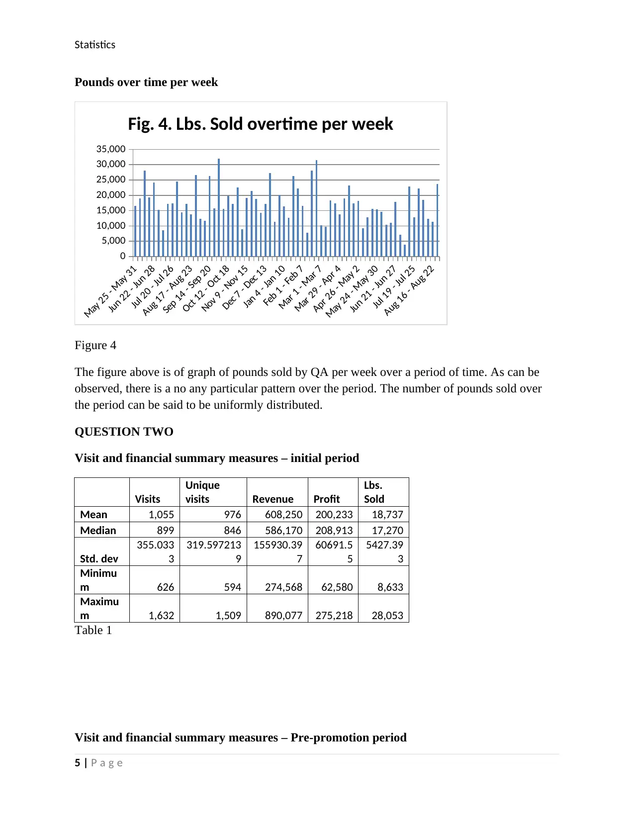
Fig. 4. Lbs. Sold overtime per week
Figure 4
The figure above is of graph of pounds sold by QA per week over a period of time. As can be
observed, there is a no any particular pattern over the period. The number of pounds sold over
the period can be said to be uniformly distributed.
QUESTION TWO
Visit and financial summary measures – initial period
Visits
Unique
visits Revenue Profit
Lbs.
Sold
Mean 1,055 976 608,250 200,233 18,737
Median 899 846 586,170 208,913 17,270
Std. dev
355.033
3
319.597213
9
155930.39
7
60691.5
5
5427.39
3
Minimu
m 626 594 274,568 62,580 8,633
Maximu
m 1,632 1,509 890,077 275,218 28,053
Table 1
Visit and financial summary measures – Pre-promotion period
5 | P a g e
Pounds over time per week
May 25 - May 31
Jun 22 - Jun 28
Jul 20 - Jul 26
Aug 17 - Aug 23
Sep 14 - Sep 20
Oct 12 - Oct 18
Nov 9 - Nov 15
Dec 7 - Dec 13
Jan 4 - Jan 10
Feb 1 - Feb 7
Mar 1 - Mar 7
Mar 29 - Apr 4
Apr 26 - May 2
May 24 - May 30
Jun 21 - Jun 27
Jul 19 - Jul 25
Aug 16 - Aug 22
0
5,000
10,000
15,000
20,000
25,000
30,000
35,000
Fig. 4. Lbs. Sold overtime per week
Figure 4
The figure above is of graph of pounds sold by QA per week over a period of time. As can be
observed, there is a no any particular pattern over the period. The number of pounds sold over
the period can be said to be uniformly distributed.
QUESTION TWO
Visit and financial summary measures – initial period
Visits
Unique
visits Revenue Profit
Lbs.
Sold
Mean 1,055 976 608,250 200,233 18,737
Median 899 846 586,170 208,913 17,270
Std. dev
355.033
3
319.597213
9
155930.39
7
60691.5
5
5427.39
3
Minimu
m 626 594 274,568 62,580 8,633
Maximu
m 1,632 1,509 890,077 275,218 28,053
Table 1
Visit and financial summary measures – Pre-promotion period
5 | P a g e
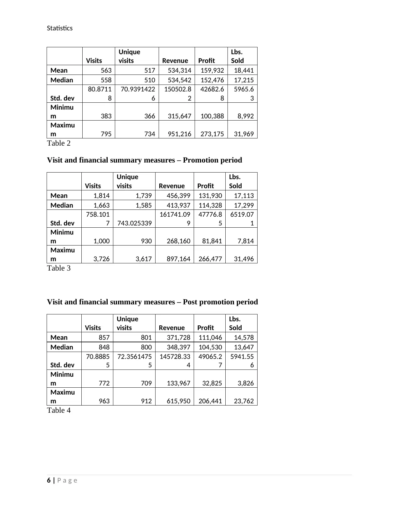
Statistics
Visits
Unique
visits Revenue Profit
Lbs.
Sold
Mean 563 517 534,314 159,932 18,441
Median 558 510 534,542 152,476 17,215
Std. dev
80.8711
8
70.9391422
6
150502.8
2
42682.6
8
5965.6
3
Minimu
m 383 366 315,647 100,388 8,992
Maximu
m 795 734 951,216 273,175 31,969
Table 2
Visit and financial summary measures – Promotion period
Visits
Unique
visits Revenue Profit
Lbs.
Sold
Mean 1,814 1,739 456,399 131,930 17,113
Median 1,663 1,585 413,937 114,328 17,299
Std. dev
758.101
7 743.025339
161741.09
9
47776.8
5
6519.07
1
Minimu
m 1,000 930 268,160 81,841 7,814
Maximu
m 3,726 3,617 897,164 266,477 31,496
Table 3
Visit and financial summary measures – Post promotion period
Visits
Unique
visits Revenue Profit
Lbs.
Sold
Mean 857 801 371,728 111,046 14,578
Median 848 800 348,397 104,530 13,647
Std. dev
70.8885
5
72.3561475
5
145728.33
4
49065.2
7
5941.55
6
Minimu
m 772 709 133,967 32,825 3,826
Maximu
m 963 912 615,950 206,441 23,762
Table 4
6 | P a g e
Visits
Unique
visits Revenue Profit
Lbs.
Sold
Mean 563 517 534,314 159,932 18,441
Median 558 510 534,542 152,476 17,215
Std. dev
80.8711
8
70.9391422
6
150502.8
2
42682.6
8
5965.6
3
Minimu
m 383 366 315,647 100,388 8,992
Maximu
m 795 734 951,216 273,175 31,969
Table 2
Visit and financial summary measures – Promotion period
Visits
Unique
visits Revenue Profit
Lbs.
Sold
Mean 1,814 1,739 456,399 131,930 17,113
Median 1,663 1,585 413,937 114,328 17,299
Std. dev
758.101
7 743.025339
161741.09
9
47776.8
5
6519.07
1
Minimu
m 1,000 930 268,160 81,841 7,814
Maximu
m 3,726 3,617 897,164 266,477 31,496
Table 3
Visit and financial summary measures – Post promotion period
Visits
Unique
visits Revenue Profit
Lbs.
Sold
Mean 857 801 371,728 111,046 14,578
Median 848 800 348,397 104,530 13,647
Std. dev
70.8885
5
72.3561475
5
145728.33
4
49065.2
7
5941.55
6
Minimu
m 772 709 133,967 32,825 3,826
Maximu
m 963 912 615,950 206,441 23,762
Table 4
6 | P a g e
⊘ This is a preview!⊘
Do you want full access?
Subscribe today to unlock all pages.
Trusted by 1+ million students worldwide
Statistics
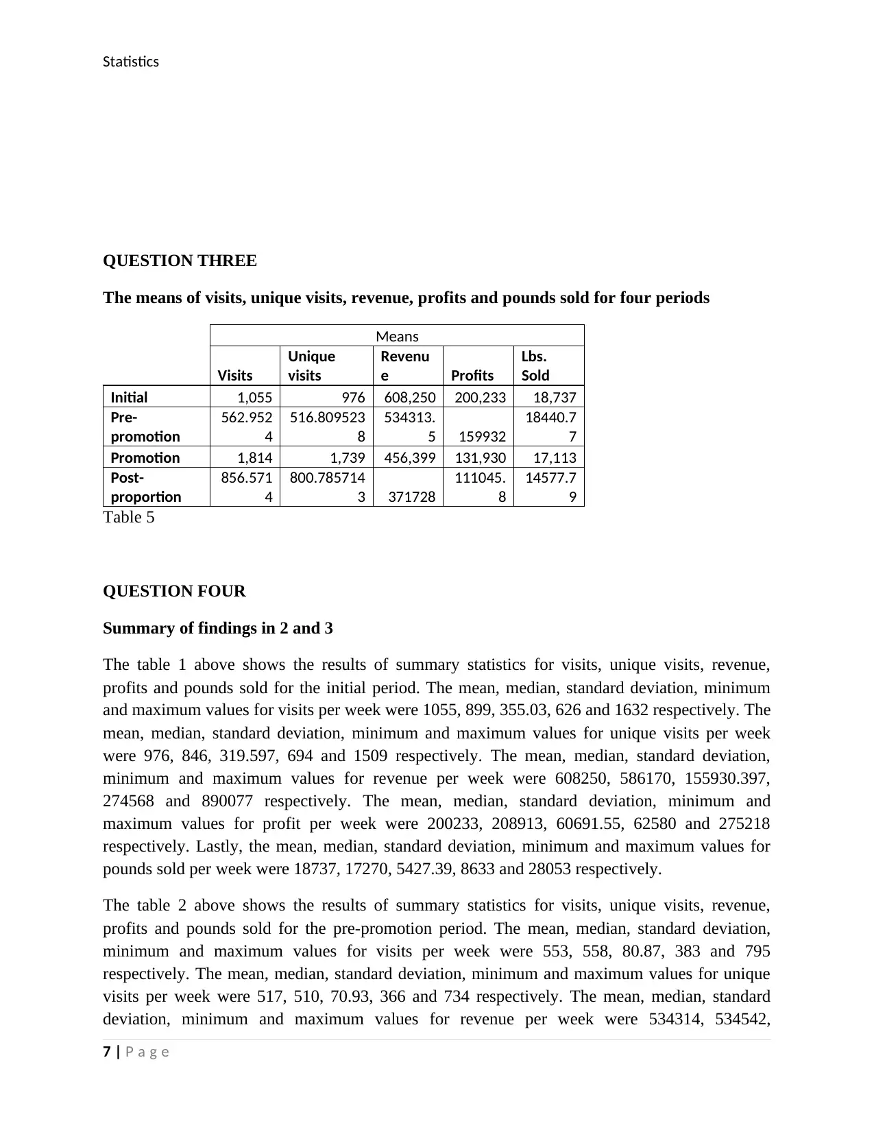
QUESTION THREE
The means of visits, unique visits, revenue, profits and pounds sold for four periods
Means
Visits
Unique
visits
Revenu
e Profits
Lbs.
Sold
Initial 1,055 976 608,250 200,233 18,737
Pre-
promotion
562.952
4
516.809523
8
534313.
5 159932
18440.7
7
Promotion 1,814 1,739 456,399 131,930 17,113
Post-
proportion
856.571
4
800.785714
3 371728
111045.
8
14577.7
9
Table 5
QUESTION FOUR
Summary of findings in 2 and 3
The table 1 above shows the results of summary statistics for visits, unique visits, revenue,
profits and pounds sold for the initial period. The mean, median, standard deviation, minimum
and maximum values for visits per week were 1055, 899, 355.03, 626 and 1632 respectively. The
mean, median, standard deviation, minimum and maximum values for unique visits per week
were 976, 846, 319.597, 694 and 1509 respectively. The mean, median, standard deviation,
minimum and maximum values for revenue per week were 608250, 586170, 155930.397,
274568 and 890077 respectively. The mean, median, standard deviation, minimum and
maximum values for profit per week were 200233, 208913, 60691.55, 62580 and 275218
respectively. Lastly, the mean, median, standard deviation, minimum and maximum values for
pounds sold per week were 18737, 17270, 5427.39, 8633 and 28053 respectively.
The table 2 above shows the results of summary statistics for visits, unique visits, revenue,
profits and pounds sold for the pre-promotion period. The mean, median, standard deviation,
minimum and maximum values for visits per week were 553, 558, 80.87, 383 and 795
respectively. The mean, median, standard deviation, minimum and maximum values for unique
visits per week were 517, 510, 70.93, 366 and 734 respectively. The mean, median, standard
deviation, minimum and maximum values for revenue per week were 534314, 534542,
7 | P a g e
Paraphrase This Document
Need a fresh take? Get an instant paraphrase of this document with our AI Paraphraser
Statistics
150502.82, 315642, and 951216 respectively. The mean, median, standard deviation, minimum
and maximum values for profit per week were 159932, 152476, 42682.68, 100388 and 273175
respectively. Lastly, the mean, median, standard deviation, minimum and maximum values for
pounds sold per week were 18441, 17215, 5965.63, 8992 and 31969 respectively.
The table 3 above shows the results of summary statistics for visits, unique visits, revenue,
profits and pounds sold for the promotion period. The mean, median, standard deviation,
minimum and maximum values for visits per week were 1814, 1663, 758.10, 1000 and 3726
respectively. The mean, median, standard deviation, minimum and maximum values for unique
visits per week were 1739, 1585, 743.02, 930 and 3617 respectively. The mean, median,
standard deviation, minimum and maximum values for revenue per week were 456399, 413937,
161741.099, 268160, and 897164 respectively. The mean, median, standard deviation, minimum
and maximum values for profit per week were 131930, 114328, 47776.85, 81841 and 266477
respectively. Lastly, the mean, median, standard deviation, minimum and maximum values for
pounds sold per week were 17113, 17229, 6519.07, 7814 and 31496 respectively.
The table 4 above shows the results of summary statistics for visits, unique visits, revenue,
profits and pounds sold for the post promotion period. The mean, median, standard deviation,
minimum and maximum values for visits per week were 857, 848, 70.89, 772 and 963
respectively. The mean, median, standard deviation, minimum and maximum values for unique
visits per week were 801, 800, 72.35, 709 and 912 respectively. The mean, median, standard
deviation, minimum and maximum values for revenue per week were 371728, 348397,
145728.33, 133967 and 615950 respectively. The mean, median, standard deviation, minimum
and maximum values for profit per week were 111046, 104530, 49065.27, 32825 and 206441
respectively. Lastly, the mean, median, standard deviation, minimum and maximum values for
pounds sold per week were 14578, 13647, 5941.56, 3826 and 23762 respectively.
It can be observed from table 5 that the mean number of visits during the initial, pre-promotion,
promotion and post promotion periods were 1055, 562.95, 1814 and 856.57. The mean number
of unique visits during the initial, pre-promotion, promotion and post promotion periods were
976, 516.81, 1739 and 800.79. The mean number of revenue during the initial, pre-promotion,
promotion and post promotion periods were 608250, 53431.5, 456339 and 371728. The mean
number of profits during the initial, pre-promotion, promotion and post promotion periods were
200233, 159932, 131930 and 111045.8. Lastly, the mean number of pounds sold during the
initial, pre-promotion, promotion and post promotion periods were 18737, 18440.77, 17113 and
14577.79
RELATIONSHIP BETWEEN VARIABLES
QUESTION FIVE
8 | P a g e
Statistics
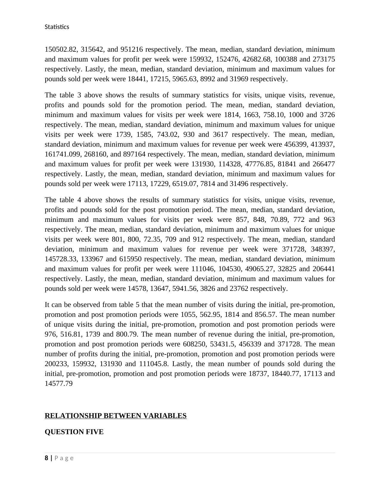
Correlation coefficient between revenue and pounds sold.
Revenu
e
Lbs.
Sold
Revenue 1
Lbs.
Sold
0.86893 1
Table 6
From my intuition, there is a positive relationship between revenue and pounds sold. This is
because any number of pounds sold can only increase the amount of revenue and not decrease.
Scatterplot of revenue versus pounds sold
0 5,000 10,000 15,000 20,000 25,000 30,000 35,000
$0
$100,000
$200,000
$300,000
$400,000
$500,000
$600,000
$700,000
$800,000
$900,000
$1,000,000
f(x) = 24.5679059575216 x + 69380.9472593738
R² = 0.755038845893767
Scatterplot of revenue vs pounds sold
Pounds sold
Revenue
Figure 5
The correlation coefficient r, between revenue and pounds sold is 0.87. This indicates that there
is a strong and positive relationship between the two variables. The scatterplot above also depicts
a linear relationship with a high value of R-squared (0.76).
Question six
Correlation of revenue versus visits
Visits Revenue
Visits 1
9 | P a g e
⊘ This is a preview!⊘
Do you want full access?
Subscribe today to unlock all pages.
Trusted by 1+ million students worldwide
Statistics
Revenu
e
-0.0593 1
Table 7
Scatterplot of revenue versus visits
0 500 1,000 1,500 2,000 2,500 3,000 3,500 4,000
$0
$100,000
$200,000
$300,000
$400,000
$500,000
$600,000
$700,000
$800,000
$900,000
$1,000,000
f(x) = − 15.970543633977 x + 512241.046258343
R² = 0.00352738952999587
Scatterplot of revenue vs visits
Visits
Revenue
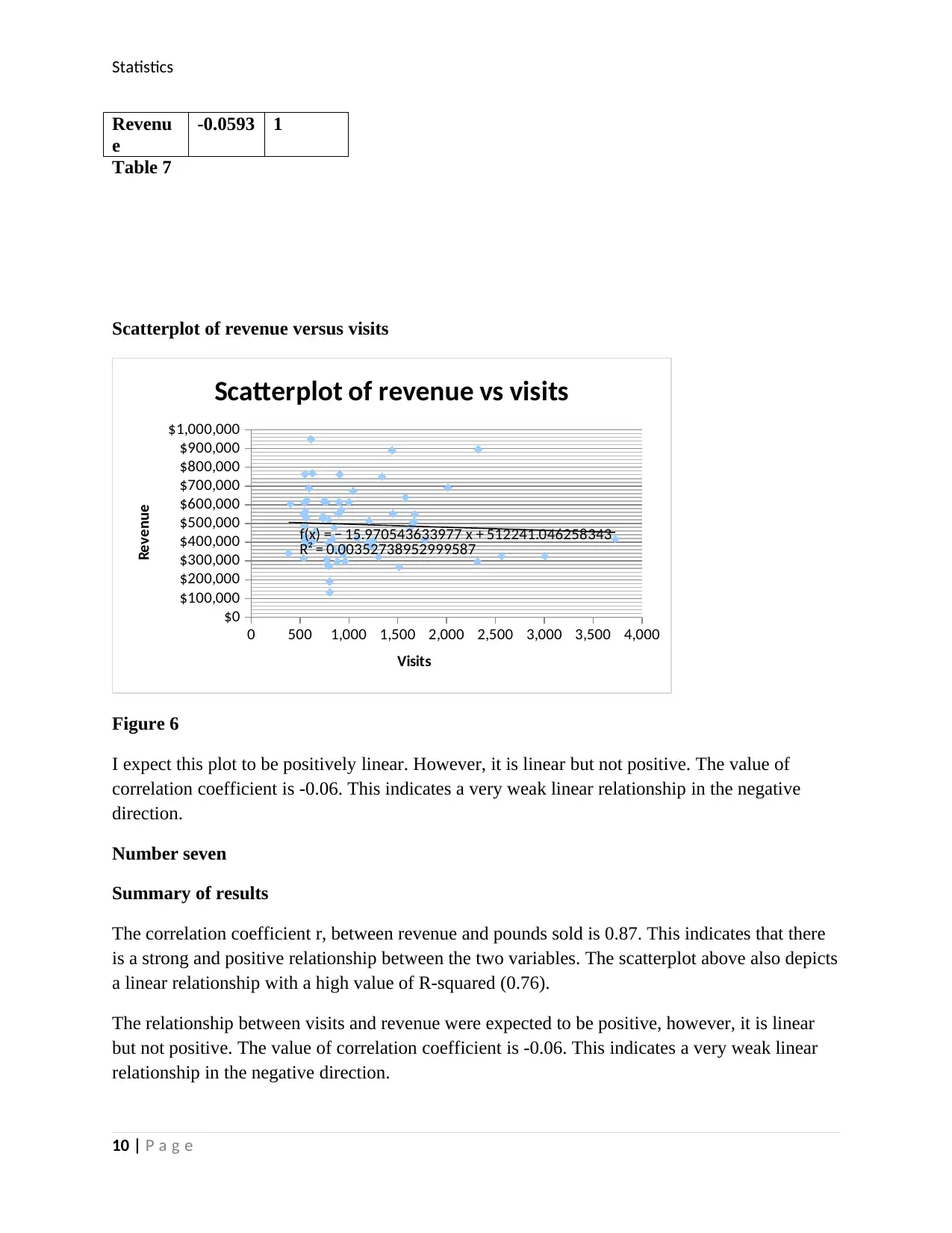
Figure 6
I expect this plot to be positively linear. However, it is linear but not positive. The value of
correlation coefficient is -0.06. This indicates a very weak linear relationship in the negative
direction.
Number seven
Summary of results
The correlation coefficient r, between revenue and pounds sold is 0.87. This indicates that there
is a strong and positive relationship between the two variables. The scatterplot above also depicts
a linear relationship with a high value of R-squared (0.76).
The relationship between visits and revenue were expected to be positive, however, it is linear
but not positive. The value of correlation coefficient is -0.06. This indicates a very weak linear
relationship in the negative direction.
10 | P a g e
Revenu
e
-0.0593 1
Table 7
Scatterplot of revenue versus visits
0 500 1,000 1,500 2,000 2,500 3,000 3,500 4,000
$0
$100,000
$200,000
$300,000
$400,000
$500,000
$600,000
$700,000
$800,000
$900,000
$1,000,000
f(x) = − 15.970543633977 x + 512241.046258343
R² = 0.00352738952999587
Scatterplot of revenue vs visits
Visits
Revenue
Figure 6
I expect this plot to be positively linear. However, it is linear but not positive. The value of
correlation coefficient is -0.06. This indicates a very weak linear relationship in the negative
direction.
Number seven
Summary of results
The correlation coefficient r, between revenue and pounds sold is 0.87. This indicates that there
is a strong and positive relationship between the two variables. The scatterplot above also depicts
a linear relationship with a high value of R-squared (0.76).
The relationship between visits and revenue were expected to be positive, however, it is linear
but not positive. The value of correlation coefficient is -0.06. This indicates a very weak linear
relationship in the negative direction.
10 | P a g e
Paraphrase This Document
Need a fresh take? Get an instant paraphrase of this document with our AI Paraphraser
Statistics
Number eight
a. Summary statistics for Lbs. sold from January 3, 2015 to January 19, 2010
Results table
Lbs. Sold
Mean
18681.5551
7
Median 17673
Standard
Deviation 6840.50794
Minimum 3826
Maximum 44740
Table 8
The summary statistics for pounds sold is as shown in the table above. The mean Lbs sold was
18681.56 while the median and the standard deviation were 17,673 and 6840.51. The minimum
and maximum number of Lbs sold was 3826 and 44740 respectively.
b. Histogram for Lbs. sold from January 3, 2015 to January 19, 2010
11 | P a g e
Statistics
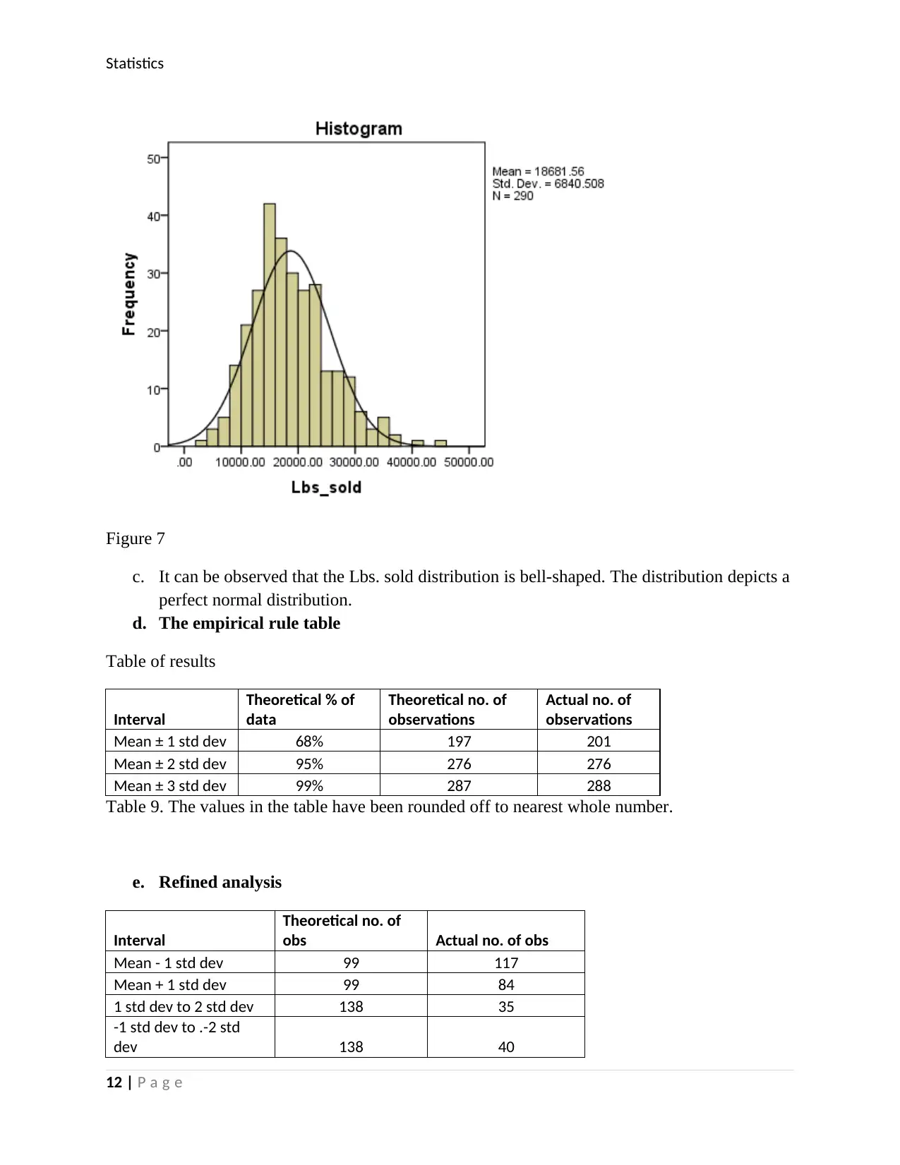
Figure 7
c. It can be observed that the Lbs. sold distribution is bell-shaped. The distribution depicts a
perfect normal distribution.
d. The empirical rule table
Table of results
Interval
Theoretical % of
data
Theoretical no. of
observations
Actual no. of
observations
Mean ± 1 std dev 68% 197 201
Mean ± 2 std dev 95% 276 276
Mean ± 3 std dev 99% 287 288
Table 9. The values in the table have been rounded off to nearest whole number.
e. Refined analysis
Interval
Theoretical no. of
obs Actual no. of obs
Mean - 1 std dev 99 117
Mean + 1 std dev 99 84
1 std dev to 2 std dev 138 35
-1 std dev to .-2 std
dev 138 40
12 | P a g e
⊘ This is a preview!⊘
Do you want full access?
Subscribe today to unlock all pages.
Trusted by 1+ million students worldwide
1 out of 19
Related Documents


Your All-in-One AI-Powered Toolkit for Academic Success.
+13062052269
info@desklib.com
Available 24*7 on WhatsApp / Email
![[object Object]](/_next/static/media/star-bottom.7253800d.svg)
Unlock your academic potential
Copyright © 2020–2026 A2Z Services. All Rights Reserved. Developed and managed by ZUCOL.