Wireless Communication: Free Space, Path Loss, and Design Analysis

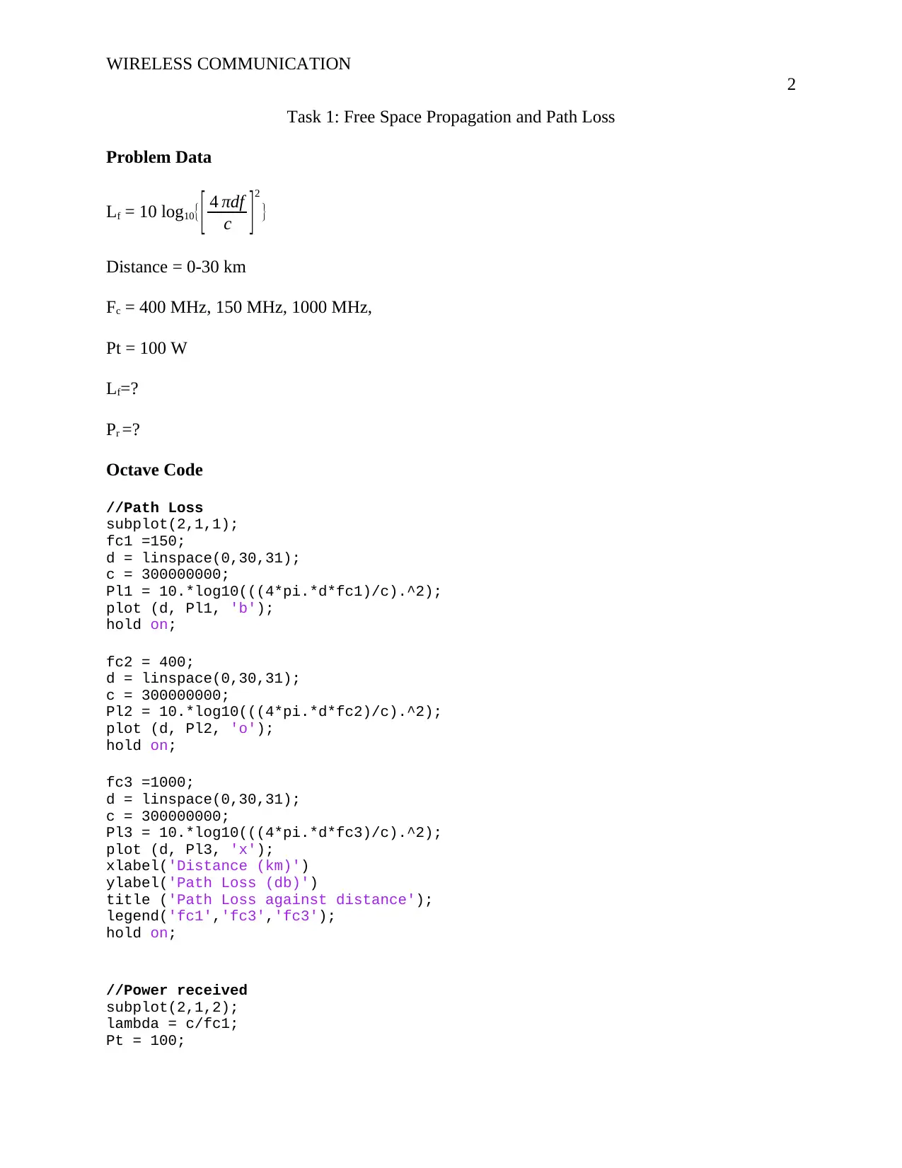
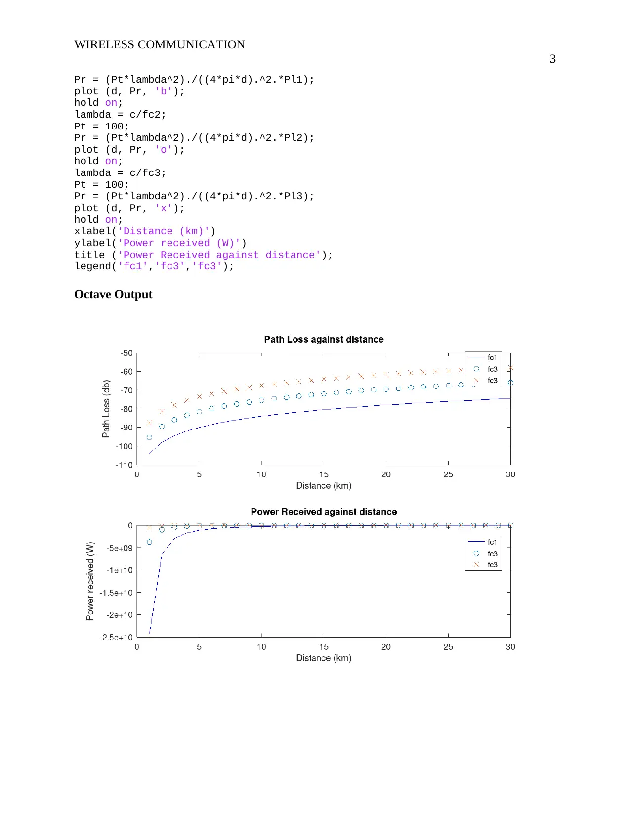
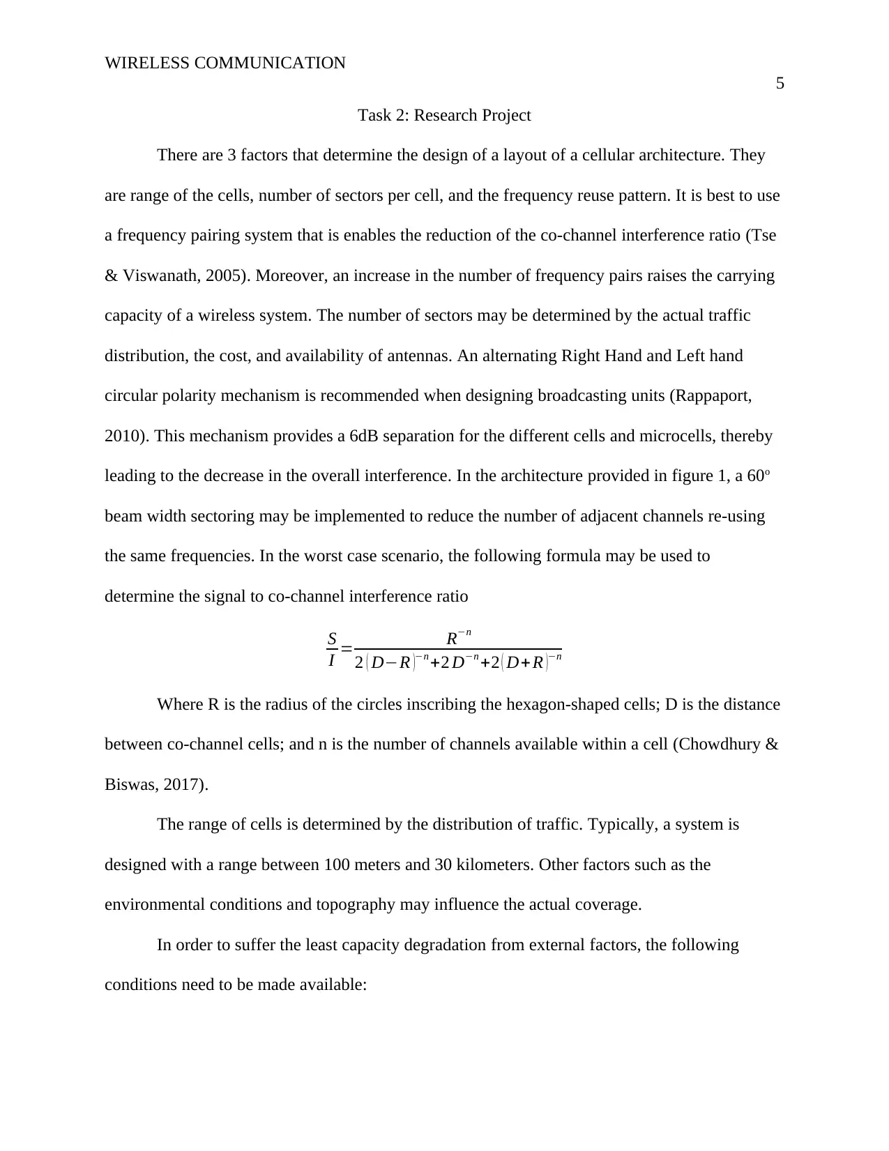
This assignment delves into the core concepts of wireless communication, encompassing two primary tasks. The first task involves analyzing free space propagation and path loss, utilizing Octave code to simulate and visualize the relationship between distance, frequency, and received power. The second task centers on the design considerations of cellular architecture, exploring factors such as cell range, sectoring, frequency reuse patterns, and the impact of antenna design. It also examines the signal-to-co-channel interference ratio and the Erlang capacity, providing a comprehensive overview of wireless communication systems. The assignment uses formulas, Octave code, and research to provide a detailed understanding of the design and implementation of wireless networks, with a focus on factors that influence coverage, interference, and capacity.

Running head: WIRELESS COMMUNICATION
1
Wireless Communication
Name
University
Date:

WIRELESS COMMUNICATION
2
Task 1: Free Space Propagation and Path Loss
Problem Data
Lf = 10 log10{
[ 4 πdf
c ]2
}
Distance = 0-30 km
Fc = 400 MHz, 150 MHz, 1000 MHz,
Pt = 100 W
Lf=?
Pr =?
Octave Code
//Path Loss
subplot(2,1,1);
fc1 =150;
d = linspace(0,30,31);
c = 300000000;
Pl1 = 10.*log10(((4*pi.*d*fc1)/c).^2);
plot (d, Pl1, 'b');
hold on;
fc2 = 400;
d = linspace(0,30,31);
c = 300000000;
Pl2 = 10.*log10(((4*pi.*d*fc2)/c).^2);
plot (d, Pl2, 'o');
hold on;
fc3 =1000;
d = linspace(0,30,31);
c = 300000000;
Pl3 = 10.*log10(((4*pi.*d*fc3)/c).^2);
plot (d, Pl3, 'x');
xlabel('Distance (km)')
ylabel('Path Loss (db)')
title ('Path Loss against distance');
legend('fc1','fc3','fc3');
hold on;
//Power received
subplot(2,1,2);
lambda = c/fc1;
Pt = 100;

WIRELESS COMMUNICATION
3
Pr = (Pt*lambda^2)./((4*pi*d).^2.*Pl1);
plot (d, Pr, 'b');
hold on;
lambda = c/fc2;
Pt = 100;
Pr = (Pt*lambda^2)./((4*pi*d).^2.*Pl2);
plot (d, Pr, 'o');
hold on;
lambda = c/fc3;
Pt = 100;
Pr = (Pt*lambda^2)./((4*pi*d).^2.*Pl3);
plot (d, Pr, 'x');
hold on;
xlabel('Distance (km)')
ylabel('Power received (W)')
title ('Power Received against distance');
legend('fc1','fc3','fc3');
Octave Output

WIRELESS COMMUNICATION
4

WIRELESS COMMUNICATION
5
Task 2: Research Project
There are 3 factors that determine the design of a layout of a cellular architecture. They
are range of the cells, number of sectors per cell, and the frequency reuse pattern. It is best to use
a frequency pairing system that is enables the reduction of the co-channel interference ratio (Tse
& Viswanath, 2005). Moreover, an increase in the number of frequency pairs raises the carrying
capacity of a wireless system. The number of sectors may be determined by the actual traffic
distribution, the cost, and availability of antennas. An alternating Right Hand and Left hand
circular polarity mechanism is recommended when designing broadcasting units (Rappaport,
2010). This mechanism provides a 6dB separation for the different cells and microcells, thereby
leading to the decrease in the overall interference. In the architecture provided in figure 1, a 60o
beam width sectoring may be implemented to reduce the number of adjacent channels re-using
the same frequencies. In the worst case scenario, the following formula may be used to
determine the signal to co-channel interference ratio
S
I = R−n
2 ( D−R )−n +2 D−n +2 ( D+R )−n
Where R is the radius of the circles inscribing the hexagon-shaped cells; D is the distance
between co-channel cells; and n is the number of channels available within a cell (Chowdhury &
Biswas, 2017).
The range of cells is determined by the distribution of traffic. Typically, a system is
designed with a range between 100 meters and 30 kilometers. Other factors such as the
environmental conditions and topography may influence the actual coverage.
In order to suffer the least capacity degradation from external factors, the following
conditions need to be made available:

WIRELESS COMMUNICATION
6
i. Utilization of directional edge-excited antennas installed at the periphery of the
desired zones, with an appropriate directivity to cover the whole region.
ii. Alternating reverse polarity of the antenna to decrease the sectoral
interferences along the borders.
The load servable within a region that marks the zoning of the cells and microcells
may be determined by the Erlang capacity, radii of the cells, type and shape of the antenna,
power of transmission, and the load density. These factors contribute to the calculation of the
height of the antenna.
The architecture in figure 1 defines an urban region, which is marked by a densely
populated central region with a dwindling Erlang number with an increase in the radius
(Takagi & Walke, 2008). The following table gives an estimate of the parameters in various
scenarios presented in the figure.
Scenario Erlang density Radius of the
Cell (km)
Area/sector
(km2)
Antenna shape
Metro 20 0.1 0.00433 Directional(60o)
Urban 12 0.5 0.10823 Directional(60o)
Suburban 8 1 0.433 Directional(60o)
Rural 4 10 314.16 Omnidirectional
(edge-excited)
The height of the antenna depends on the terrain of the region as well as the location,
whether on a static or mobile unit. The effective height of an antenna on a hill is the sum of the
height of the hill and the height of the antenna. (h+H). In a valley, the effective height is 1/6 of
the total valley height. ( 1
6 h)
A reduction in the gain of the antenna causes a reduction in the height.
G = 20 log 10 0.5 h+ H
h+H

WIRELESS COMMUNICATION
7
From the above discussion, the number of base stations required to cover the whole
region are 4 — One at the central location and 3 at a 120o spread along the periphery of the zone.

WIRELESS COMMUNICATION
8
References
Chowdhury, M., & Biswas, A. (2017). Wireless Communication: Theory and Applications.
Cambridge University Press.
Rappaport, T. S. (2010). Wireless Communications: Principles And Practice, 2/E. Pearson
Education India.
Takagi, H., & Walke, B. H. (2008). Spectrum Requirement Planning in Wireless
Communications: Model and Methodology for IMT - Advanced. John Wiley & Sons.
Tse, D., & Viswanath, P. (2005). Fundamentals of Wireless Communication. Cambridge
University Press.