Math 15: Income, Education, and Depression Analysis using WLS Dataset

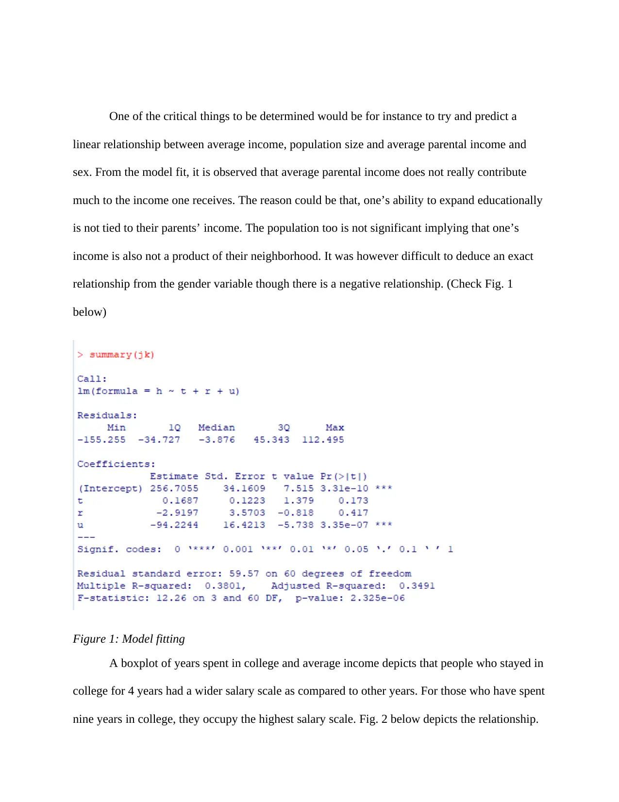
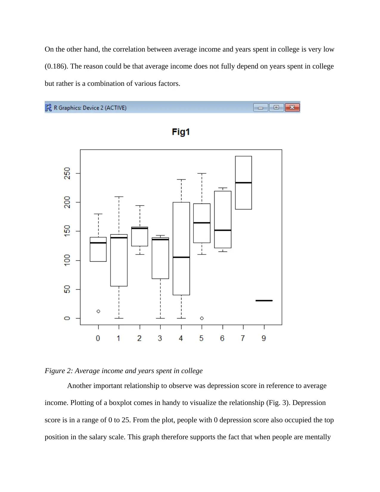
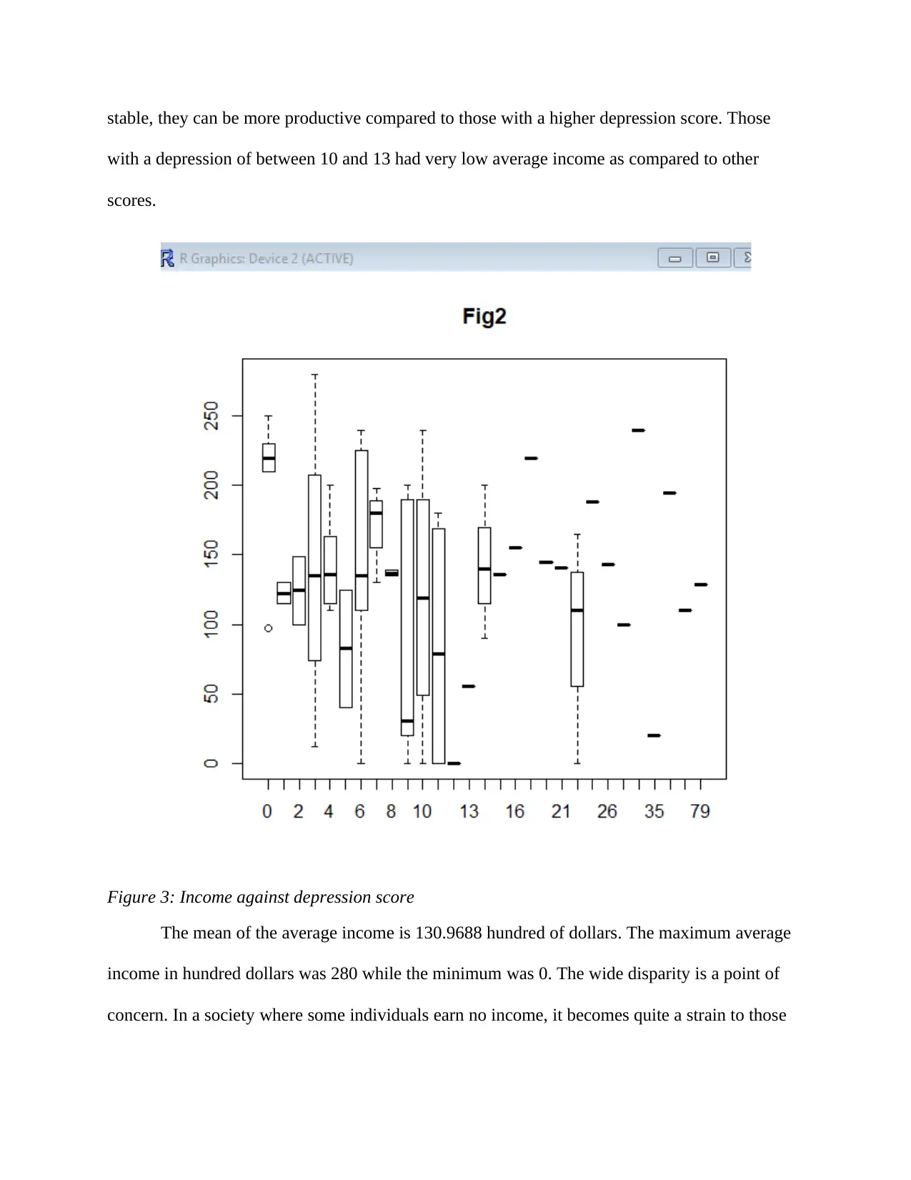
This assignment analyzes the WLS dataset, focusing on the relationships between income, education, and depression scores. The analysis reveals that parental income and population size have an insignificant impact on an individual's income, while gender shows a negative correlation. The years spent in college show a positive correlation with income, with those spending four or nine years in college having a wider salary scale and the highest salary scale, respectively, although the correlation is weak. Furthermore, the analysis indicates that individuals with a depression score of 0 occupy the top position in the salary scale, suggesting a positive correlation between mental stability and income. The assignment also provides statistical summaries of income, including mean, maximum, and minimum values, highlighting income disparity and the adequacy of a model with intercept only, based on ANOVA results. The student used the WLS dataset to explore relationships between income, education, and health.

One of the critical things to be determined would be for instance to try and predict a
linear relationship between average income, population size and average parental income and
sex. From the model fit, it is observed that average parental income does not really contribute
much to the income one receives. The reason could be that, one’s ability to expand educationally
is not tied to their parents’ income. The population too is not significant implying that one’s
income is also not a product of their neighborhood. It was however difficult to deduce an exact
relationship from the gender variable though there is a negative relationship. (Check Fig. 1
below)
Figure 1: Model fitting
A boxplot of years spent in college and average income depicts that people who stayed in
college for 4 years had a wider salary scale as compared to other years. For those who have spent
nine years in college, they occupy the highest salary scale. Fig. 2 below depicts the relationship.

On the other hand, the correlation between average income and years spent in college is very low
(0.186). The reason could be that average income does not fully depend on years spent in college
but rather is a combination of various factors.
Figure 2: Average income and years spent in college
Another important relationship to observe was depression score in reference to average
income. Plotting of a boxplot comes in handy to visualize the relationship (Fig. 3). Depression
score is in a range of 0 to 25. From the plot, people with 0 depression score also occupied the top
position in the salary scale. This graph therefore supports the fact that when people are mentally

stable, they can be more productive compared to those with a higher depression score. Those
with a depression of between 10 and 13 had very low average income as compared to other
scores.
Figure 3: Income against depression score
The mean of the average income is 130.9688 hundred of dollars. The maximum average
income in hundred dollars was 280 while the minimum was 0. The wide disparity is a point of
concern. In a society where some individuals earn no income, it becomes quite a strain to those

close to them. It might hinder development in some cases. A model is an important tool used in
projection of a certain factor based on other variables. It is often represented in an equation form.
To test adequacy of a model, ANOVA is used. In the model shown above, it can be
concluded that a model without the variables is a better fit compared to the model with variables
at 5% significance level. The null hypothesis rejected and it is concluded that the model is good
with intercept. ANOVA is handy in testing hypothesis as well. The null hypothesis is that model
is not good with intercept only against alternative hypothesis that model is good with intercept
only. A model not good with intercept only appreciates the contribution other variables have in
the model. The residual deviance statistic is used which is compared to a tabulated chi-square
value to form a basis of rejecting or failing to reject. In this case the residual deviance was
greater than tabulated value hence rejection of the null hypothesis.