Control System Robot Arm Control System
VerifiedAdded on 2023/03/31
|30
|3996
|339
AI Summary
This document discusses the control system of a robot arm control system. It covers topics such as calculating the closed loop system characteristic equation, finding the range of gain k for stability using Jury test, Nyquist method, and root locus method. It also includes the design of a lead compensator using the Reaction curve method of Ziegler-Nichols tuning.
Contribute Materials
Your contribution can guide someone’s learning journey. Share your
documents today.

1
Student
Instructor
Control system
Date
Student
Instructor
Control system
Date
Secure Best Marks with AI Grader
Need help grading? Try our AI Grader for instant feedback on your assignments.
2
QUESTION 1
The system below shows a robot arm control system. Assuming the sampling time Ts=0.1s and
assuming the digital controller transfer function is D(z)=1. Calculating the following
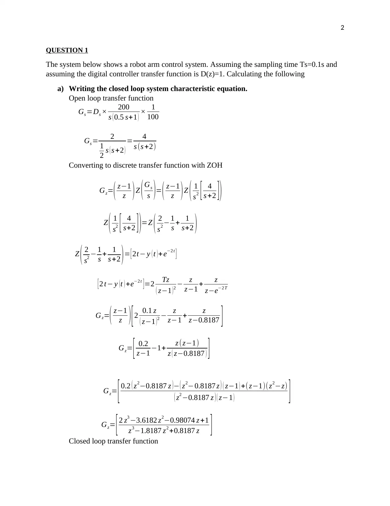
a) Writing the closed loop system characteristic equation.
Open loop transfer function
Gs =Ds × 200
s ( 0.5 s+1 ) × 1
100
Gs = 2
1
2 s ( s +2 )
= 4
s (s +2)
Converting to discrete transfer function with ZOH
Gz=( z−1
z )Z (Gs
s )= ( z−1
z )Z ( 1
s2 [ 4
s +2 ])
Z ( 1
s2 [ 4
s+2 ] )=Z ( 2
s2 − 1
s + 1
s+2 )
Z ( 2
s2 − 1
s + 1
s +2 )= [ 2t− y ( t )+ e−2 t ]
[ 2 t− y ( t ) +e−2 t ] =2 Tz
( z−1 ) 2 − z
z−1 + z
z−e−2 T
Gz=( z−1
z ) [ 2 0.1 z
( z−1 ) 2 − z
z−1 + z
z−0.8187 ]
Gz= [ 0.2
z−1 −1+ z (z−1)
z ( z−0.8187 ) ]
Gz= [ 0.2 ( z2−0.8187 z )− ( z2−0.8187 z ) ( z−1 ) +( z−1)(z2−z)
( z2 −0.8187 z ) ( z−1 ) ]
Gz= [ 2 z3 −3.6182 z2−0.98074 z +1
z3−1.8187 z2 +0.8187 z ]
Closed loop transfer function
QUESTION 1
The system below shows a robot arm control system. Assuming the sampling time Ts=0.1s and
assuming the digital controller transfer function is D(z)=1. Calculating the following
a) Writing the closed loop system characteristic equation.
Open loop transfer function
Gs =Ds × 200
s ( 0.5 s+1 ) × 1
100
Gs = 2
1
2 s ( s +2 )
= 4
s (s +2)
Converting to discrete transfer function with ZOH
Gz=( z−1
z )Z (Gs
s )= ( z−1
z )Z ( 1
s2 [ 4
s +2 ])
Z ( 1
s2 [ 4
s+2 ] )=Z ( 2
s2 − 1
s + 1
s+2 )
Z ( 2
s2 − 1
s + 1
s +2 )= [ 2t− y ( t )+ e−2 t ]
[ 2 t− y ( t ) +e−2 t ] =2 Tz
( z−1 ) 2 − z
z−1 + z
z−e−2 T
Gz=( z−1
z ) [ 2 0.1 z
( z−1 ) 2 − z
z−1 + z
z−0.8187 ]
Gz= [ 0.2
z−1 −1+ z (z−1)
z ( z−0.8187 ) ]
Gz= [ 0.2 ( z2−0.8187 z )− ( z2−0.8187 z ) ( z−1 ) +( z−1)(z2−z)
( z2 −0.8187 z ) ( z−1 ) ]
Gz= [ 2 z3 −3.6182 z2−0.98074 z +1
z3−1.8187 z2 +0.8187 z ]
Closed loop transfer function
3
Gz−cl= k . Gz
1+k . H .Gz
= k . Gz
1+0.7 k .Gz
Gz−cl=
k . [ 2 z3−3.6182 z2−0.98074 z+1
z3 −1.8187 z2 +0.8187 z ]
1+0.07 k . [ 2 z3−3.6182 z2−0.98074 z +1
z3−1.8187 z2+ 0.8187 z ]
Gz−cl= k . ( 2 z3−3.6182 z2 −0.98074 z+ 1 )
( z3−1.8187 z2 +0.8187 z ) +0.07 k . ( 2 z3−3.6182 z2−0.98074 z +1 )
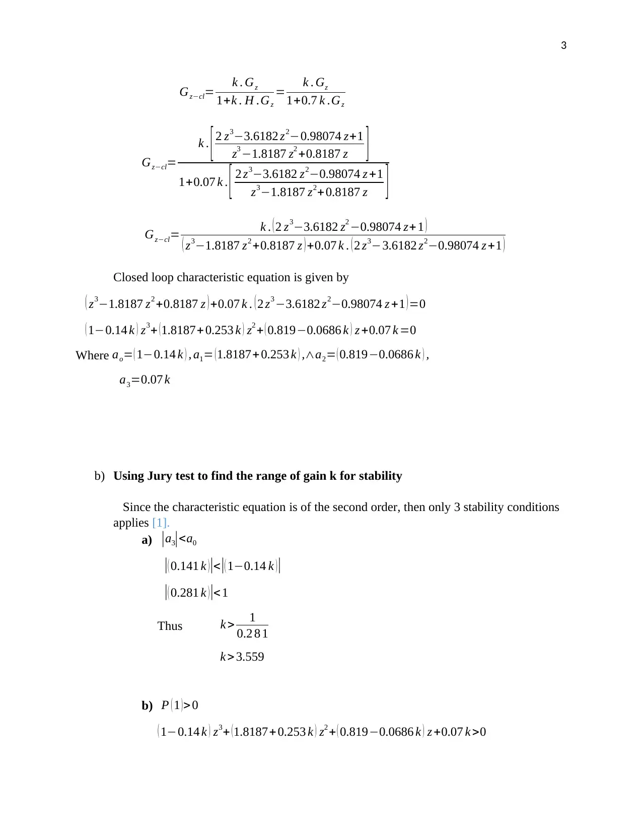
Closed loop characteristic equation is given by
( z3−1.8187 z2 +0.8187 z ) +0.07 k . ( 2 z3 −3.6182 z2−0.98074 z +1 ) =0
( 1−0.14 k ) z3+ (1.8187+ 0.253 k ) z2 + ( 0.819−0.0686 k ) z +0.07 k =0
Where ao= ( 1−0.14 k ) , a1= ( 1.8187+ 0.253 k ) ,∧a2= ( 0.819−0.0686 k ) ,
a3=0.07 k
b) Using Jury test to find the range of gain k for stability
Since the characteristic equation is of the second order, then only 3 stability conditions
applies [1].
a) |a3|<a0
|( 0.141 k )|<|( 1−0.14 k )|
|( 0.281 k )|< 1
Thus k > 1
0.2 8 1
k > 3.559
b) P ( 1 )>0
( 1−0.14 k ) z3+ (1.8187+ 0.253 k ) z2 + ( 0.819−0.0686 k ) z +0.07 k >0
Gz−cl= k . Gz
1+k . H .Gz
= k . Gz
1+0.7 k .Gz
Gz−cl=
k . [ 2 z3−3.6182 z2−0.98074 z+1
z3 −1.8187 z2 +0.8187 z ]
1+0.07 k . [ 2 z3−3.6182 z2−0.98074 z +1
z3−1.8187 z2+ 0.8187 z ]
Gz−cl= k . ( 2 z3−3.6182 z2 −0.98074 z+ 1 )
( z3−1.8187 z2 +0.8187 z ) +0.07 k . ( 2 z3−3.6182 z2−0.98074 z +1 )
Closed loop characteristic equation is given by
( z3−1.8187 z2 +0.8187 z ) +0.07 k . ( 2 z3 −3.6182 z2−0.98074 z +1 ) =0
( 1−0.14 k ) z3+ (1.8187+ 0.253 k ) z2 + ( 0.819−0.0686 k ) z +0.07 k =0
Where ao= ( 1−0.14 k ) , a1= ( 1.8187+ 0.253 k ) ,∧a2= ( 0.819−0.0686 k ) ,
a3=0.07 k
b) Using Jury test to find the range of gain k for stability
Since the characteristic equation is of the second order, then only 3 stability conditions
applies [1].
a) |a3|<a0
|( 0.141 k )|<|( 1−0.14 k )|
|( 0.281 k )|< 1
Thus k > 1
0.2 8 1
k > 3.559
b) P ( 1 )>0
( 1−0.14 k ) z3+ (1.8187+ 0.253 k ) z2 + ( 0.819−0.0686 k ) z +0.07 k >0
4
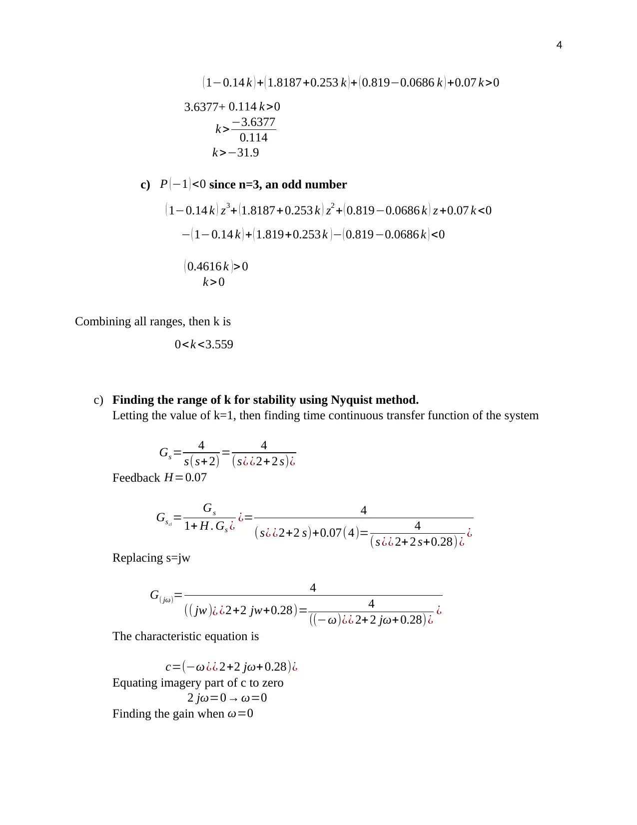
( 1−0.14 k ) + ( 1.8187+0.253 k )+ ( 0.819−0.0686 k ) +0.07 k >0
3.6377+ 0.114 k >0
k > −3.6377
0.114
k >−31.9
c) P (−1 ) <0 since n=3, an odd number
( 1−0.14 k ) z3+ (1.8187+ 0.253 k ) z2 + ( 0.819−0.0686 k ) z +0.07 k <0
− ( 1−0.14 k ) + ( 1.819+0.253 k )− ( 0.819−0.0686 k ) <0
( 0.4616 k )> 0
k > 0
Combining all ranges, then k is
0<k <3.559
c) Finding the range of k for stability using Nyquist method.
Letting the value of k=1, then finding time continuous transfer function of the system
Gs = 4
s(s+2) = 4
(s¿ ¿2+ 2 s)¿
Feedback H=0.07
Gscl
= Gs
1+ H . Gs ¿ ¿= 4
( s¿ ¿2+2 s)+0.07(4)= 4
( s ¿¿ 2+ 2 s+0.28)¿ ¿
Replacing s=jw
G( jω)= 4
(( jw )¿ ¿2+2 jw+0.28)= 4
((−ω)¿¿ 2+ 2 jω+0.28)¿ ¿
The characteristic equation is
c=(−ω ¿¿ 2+2 jω+0.28)¿
Equating imagery part of c to zero
2 jω=0→ ω=0
Finding the gain when ω=0
Secure Best Marks with AI Grader
Need help grading? Try our AI Grader for instant feedback on your assignments.
5
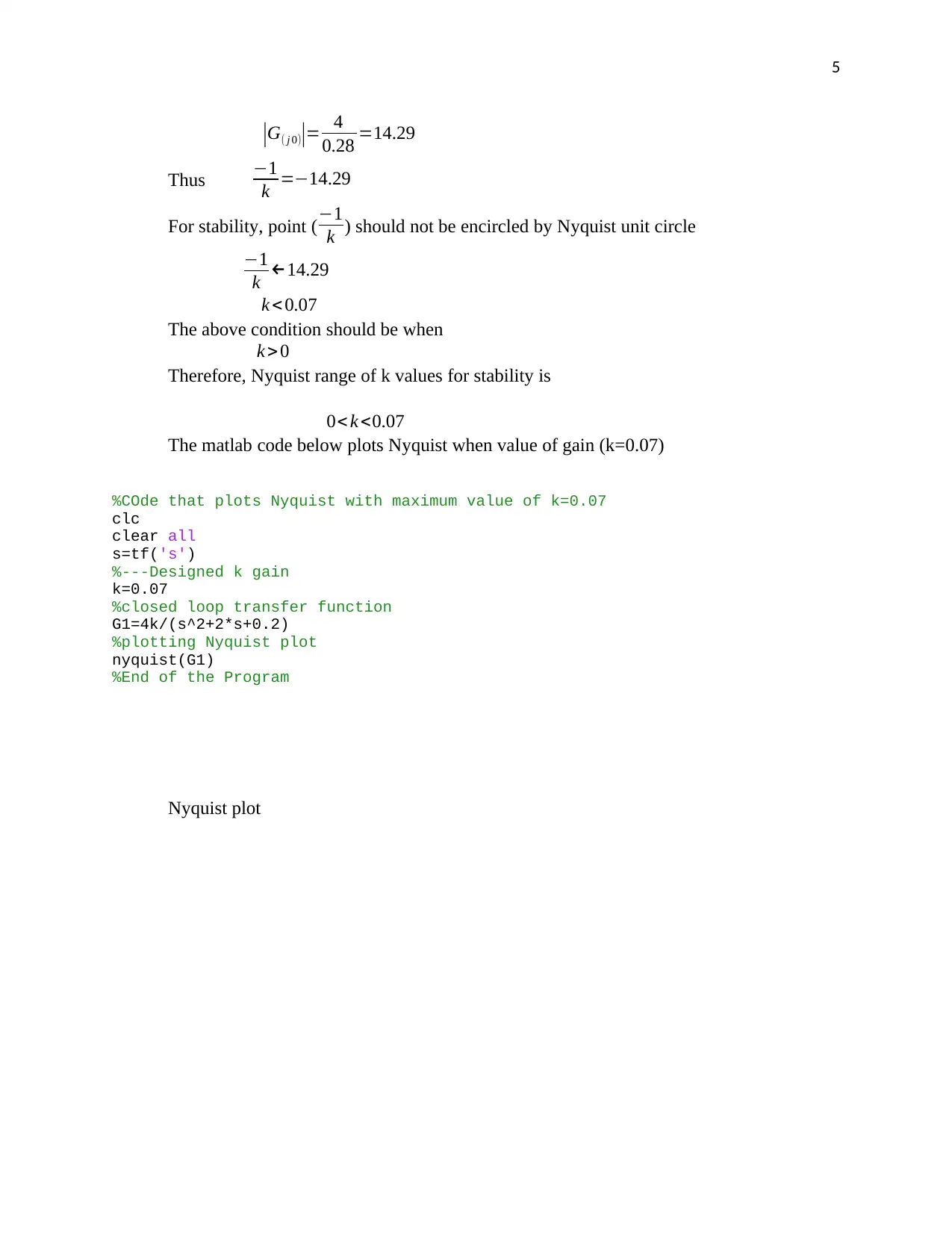
|G( j 0)|= 4
0.28 =14.29
Thus −1
k =−14.29
For stability, point (−1
k ) should not be encircled by Nyquist unit circle
−1
k ←14.29
k <0.07
The above condition should be when
k >0
Therefore, Nyquist range of k values for stability is
0< k <0.07
The matlab code below plots Nyquist when value of gain (k=0.07)
%COde that plots Nyquist with maximum value of k=0.07
clc
clear all
s=tf('s')
%---Designed k gain
k=0.07
%closed loop transfer function
G1=4k/(s^2+2*s+0.2)
%plotting Nyquist plot
nyquist(G1)
%End of the Program
Nyquist plot
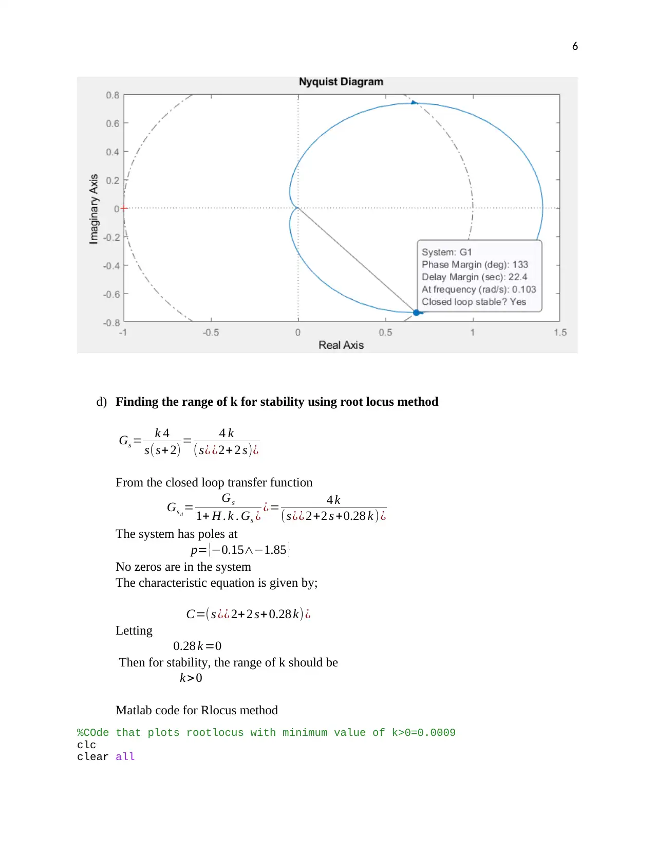
6
d) Finding the range of k for stability using root locus method
Gs = k 4
s(s+2) = 4 k
( s¿ ¿2+ 2 s)¿
From the closed loop transfer function
Gscl
= Gs
1+ H . k . Gs ¿ ¿= 4 k
(s¿¿ 2+2 s +0.28 k ) ¿
The system has poles at
p= {−0.15∧−1.85 }
No zeros are in the system
The characteristic equation is given by;
C=(s ¿¿ 2+ 2 s+0.28 k) ¿
Letting
0.28 k =0
Then for stability, the range of k should be
k >0
Matlab code for Rlocus method
%COde that plots rootlocus with minimum value of k>0=0.0009
clc
clear all
7
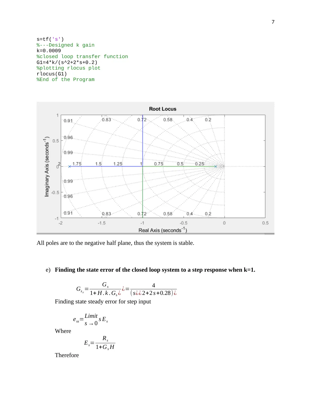
s=tf('s')
%---Designed k gain
k=0.0009
%closed loop transfer function
G1=4*k/(s^2+2*s+0.2)
%plotting rlocus plot
rlocus(G1)
%End of the Program
All poles are to the negative half plane, thus the system is stable.
e) Finding the state error of the closed loop system to a step response when k=1.
Gscl
= Gs
1+ H . k . Gs ¿ ¿= 4
( s¿¿ 2+2 s +0.28)¿
Finding state steady error for step input
ess=Limit
s →0 s Es
Where
Es= Rs
1+Gs H
Therefore
Paraphrase This Document
Need a fresh take? Get an instant paraphrase of this document with our AI Paraphraser
8
ess=Limit
s →0 s Rs
1+Gs H =s
1
s
¿ ¿
ess=Limit
s →0 s Rs
1+Gs H =(s¿¿ 2+2 s +0.28)
¿ ¿ ¿
ess=0.065
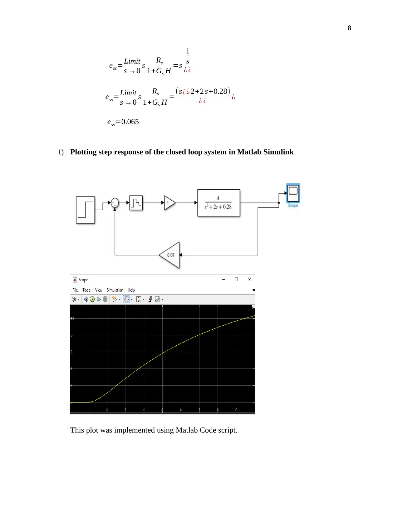
f) Plotting step response of the closed loop system in Matlab Simulink
This plot was implemented using Matlab Code script.
ess=Limit
s →0 s Rs
1+Gs H =s
1
s
¿ ¿
ess=Limit
s →0 s Rs
1+Gs H =(s¿¿ 2+2 s +0.28)
¿ ¿ ¿
ess=0.065
f) Plotting step response of the closed loop system in Matlab Simulink
This plot was implemented using Matlab Code script.
9
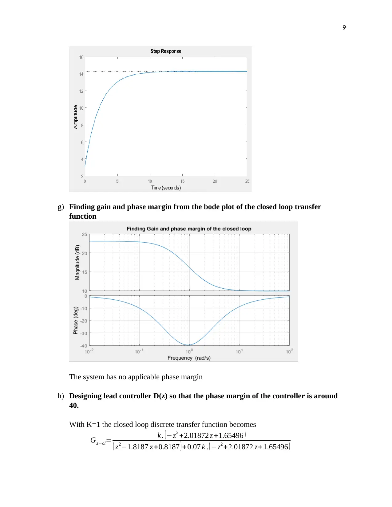
g) Finding gain and phase margin from the bode plot of the closed loop transfer
function
The system has no applicable phase margin
h) Designing lead controller D(z) so that the phase margin of the controller is around
40.
With K=1 the closed loop discrete transfer function becomes
Gz−cl= k . (−z2 +2.01872 z +1.65496 )
( z2−1.8187 z +0.8187 ) + 0.07 k . ( −z2 +2.01872 z+ 1.65496 )
10
Gz−cl= ( −z2+2.01872 z+ 1.65496 )
( z2−1.8187 z +0.8187 ) + ( −0.07 z2+0.141 z +0.1158 )
Gz−cl= (−z2 +2.01872 z+1.65496 )
(0.9345 z2−1.678 z+ 0.9345 )
Solving numerator quadratic equation (−z2+ 2.01872 z +1.65496), the system has zeros at
z=2.64∧z=−0.626
Also, solving the characteristic equation ( 0.9345 z2−1.678 z+ 0.9345), the system has
poles at
z=0.9+ j 0.44∧z =0.9− j0.44
The system has complex poles.
General equation of lead compensator is as shown below
Dz=k z−b
z−a where 0< a<b<1
Since the controller is used to improve the transient response of the system, then the d.c
gain of the lead controller must be close to 1 so as not to affect the steady state response,
D(1 )=1
Poles located in the left half plane ( z=0.9+ j 0.44 z=0.9− j 0.44) cause system to be
unstable and can be resolved by making zeros of the compensator close to z=0.9
Dz=k z−b
z−a →b=0.89 , a=0.85
Dz=k z−0.89
z−0.85
Finding value of k
D(1 )=k 1−0.89
1−0.85 =1
k = 1
0.733 1.36
The lead compensator designed is
Dz=1.36 z−0.89
z−0.85
QUESTION 2
The transfer function of motor and amplifier has been given
a. Finding a discrete time PID controller using Reaction curve method of
Ziegler-Nichols tuning and plotting the step response of the controller
Secure Best Marks with AI Grader
Need help grading? Try our AI Grader for instant feedback on your assignments.
11
Gp ( s )= 20
(s+ 1)(s+5) and GA ( s )= 0.5
(2 s+ 1)
Finding the combined closed loop system characteristic equation
C=1+Gp ( s ) GA (s ) (Kc)
Where ( Kc ) is thecontroller
C=1+ [ 20
( s +1 ) ( s+ 5 ) ][ 0.5
( 2 s +1 ) ] ( K c ) =0
C= 10(K c)
2 s3 +13 s2 +16 s +5 +1=0
C=2 s3+13 s2+16 s+5+10 KCU =0
Substituting s=jw
C=2( jω)3 +13( jω)2 +16( jω)+5+10 ¿
−2 j ω3 −13 ω2 +16( jω)+(5+10 KCU )=0
Finding w by solving imagery part
−2 j ω3 +16 ( jω )=0
ω= √ 16
2 = √ 8
Finding ultimate period time
Pu= 2 π
ω = 2 π
√8 =2.22
Finding gain Kcu by solving real part
−13 ω2+5+10 KCU =0
−13 ( 8 ) +5+10 KCU =0
10 Kc=99 → KCU=9.9
From Zieglar PID tuning table
Kp τ I τ d
PID KCU
1.7
PU
2
PU
8
12
5.62 1.11 0.2775
Time continuous PID controller designed
PID=k p (1+ τ I
s + τd s )=5.62 (1+ 1.11
s +0.2775 s )
The following Matlab code converts PID controller into digital form and plots step response of
the system
%BEGINNING OF THE CODE
clc
clear all
s=tf('s');
%Transfer function of the motor
Gp=20/((s+1)*(s+5))
%Transfer function of the amplifier
Ga=0.5/(2*s+1);
%Open loop transfer function
Gss=Ga*Gp;
%Designed constants of PID controller using reaction curve Ziegler
%--Nichols tuning
kp=5.94;
ti=5.35;
td=1.65;
%--Transfer function of the designed PID
PID=kp*(1+ti/s+td*s)
%Conversion to Dicrete
Ts=0.002 % Sampling period
PIDz=c2d(PID,Ts,'tustin')
%CLosed loop transfer function of the system
Gf=feedback(Gss*PID,1);
%Step response of the closed loop system
step(Gf)
stepinfo(Gf)
%END OF THE CODE
Digitized PID is
PIDd = 9807 z2 −1.96e04 z+ 9795
z2−1
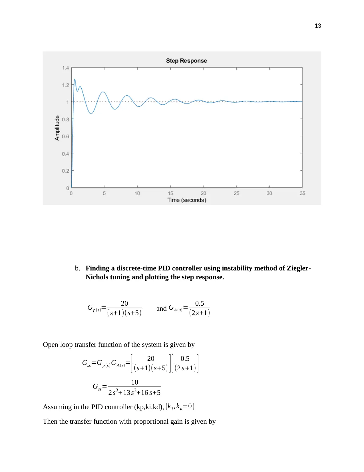
Step response of the closed loop
5.62 1.11 0.2775
Time continuous PID controller designed
PID=k p (1+ τ I
s + τd s )=5.62 (1+ 1.11
s +0.2775 s )
The following Matlab code converts PID controller into digital form and plots step response of
the system
%BEGINNING OF THE CODE
clc
clear all
s=tf('s');
%Transfer function of the motor
Gp=20/((s+1)*(s+5))
%Transfer function of the amplifier
Ga=0.5/(2*s+1);
%Open loop transfer function
Gss=Ga*Gp;
%Designed constants of PID controller using reaction curve Ziegler
%--Nichols tuning
kp=5.94;
ti=5.35;
td=1.65;
%--Transfer function of the designed PID
PID=kp*(1+ti/s+td*s)
%Conversion to Dicrete
Ts=0.002 % Sampling period
PIDz=c2d(PID,Ts,'tustin')
%CLosed loop transfer function of the system
Gf=feedback(Gss*PID,1);
%Step response of the closed loop system
step(Gf)
stepinfo(Gf)
%END OF THE CODE
Digitized PID is
PIDd = 9807 z2 −1.96e04 z+ 9795
z2−1
Step response of the closed loop
13
b. Finding a discrete-time PID controller using instability method of Ziegler-
Nichols tuning and plotting the step response.
Gp (s)= 20
( s+1)(s+5) and GA (s)= 0.5
(2 s+1)
Open loop transfer function of the system is given by
Gss=Gp (s) GA (s)= [ 20
(s +1)(s+5) ][ 0.5
(2 s +1) ]
Gss= 10
2 s3+ 13 s2+16 s+5
Assuming in the PID controller (kp,ki,kd), ( k i , k d=0 )
Then the transfer function with proportional gain is given by
Paraphrase This Document
Need a fresh take? Get an instant paraphrase of this document with our AI Paraphraser
14
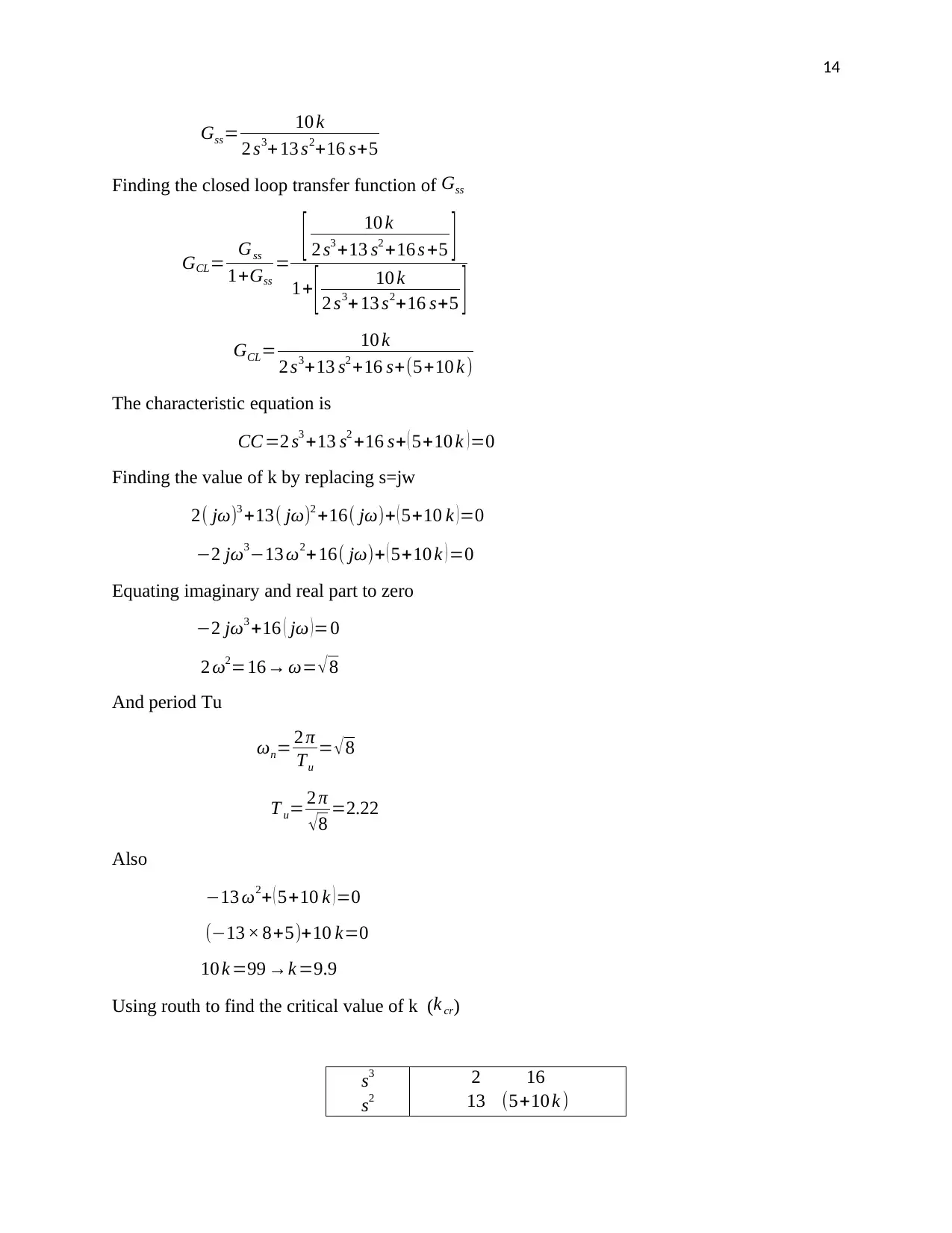
Gss= 10 k
2 s3+13 s2+16 s+5
Finding the closed loop transfer function of Gss
GCL= Gss
1+Gss
= [ 10 k
2 s3 +13 s2 +16 s +5 ]
1+ [ 10 k
2 s3+ 13 s2+16 s+5 ]
GCL= 10 k
2 s3+13 s2 +16 s+(5+10 k )
The characteristic equation is
CC =2 s3 +13 s2 +16 s+ ( 5+10 k ) =0
Finding the value of k by replacing s=jw
2( jω)3 +13( jω)2 +16( jω)+ ( 5+10 k )=0
−2 jω3−13 ω2+16( jω)+ ( 5+10 k ) =0
Equating imaginary and real part to zero
−2 jω3 +16 ( jω )=0
2 ω2=16→ ω= √ 8
And period Tu
ωn= 2 π
Tu
= √8
T u= 2 π
√8 =2.22
Also
−13 ω2+ ( 5+10 k )=0
(−13 × 8+5)+10 k=0
10 k =99 →k =9.9
Using routh to find the critical value of k (k cr)
s3
s2
2 16
13 (5+10 k )
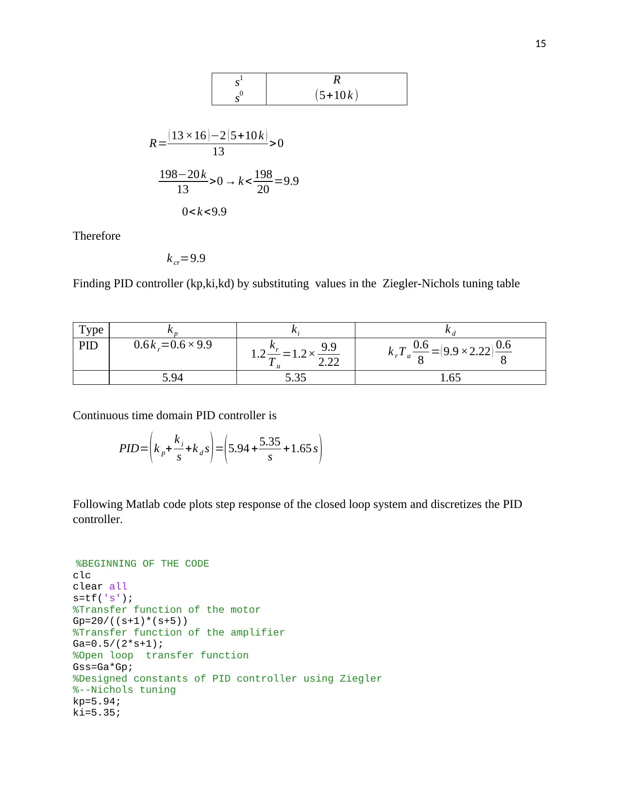
15
s1
s0
R
(5+10 k )
R= ( 13 ×16 )−2 ( 5+10 k )
13 > 0
198−20 k
13 >0 → k < 198
20 =9.9
0< k <9.9
Therefore
k cr=9.9
Finding PID controller (kp,ki,kd) by substituting values in the Ziegler-Nichols tuning table
Type k p ki k d
PID 0.6 k r=0.6 × 9.9 1.2 kr
T u
=1.2× 9.9
2.22 k r T u
0.6
8 = ( 9.9 ×2.22 ) 0.6
8
5.94 5.35 1.65
Continuous time domain PID controller is
PID= (k p+ k i
s +k d s )=(5.94 + 5.35
s +1.65 s )
Following Matlab code plots step response of the closed loop system and discretizes the PID
controller.
%BEGINNING OF THE CODE
clc
clear all
s=tf('s');
%Transfer function of the motor
Gp=20/((s+1)*(s+5))
%Transfer function of the amplifier
Ga=0.5/(2*s+1);
%Open loop transfer function
Gss=Ga*Gp;
%Designed constants of PID controller using Ziegler
%--Nichols tuning
kp=5.94;
ki=5.35;
16
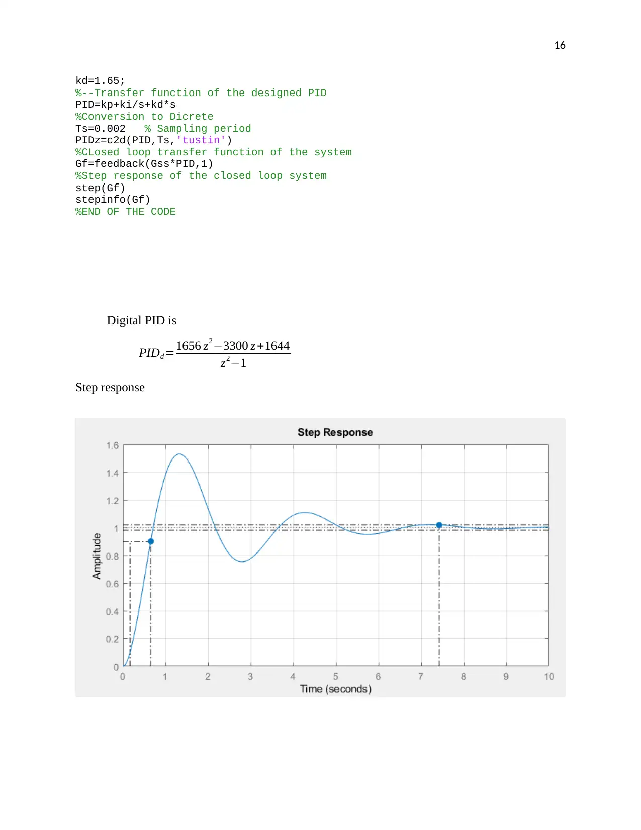
kd=1.65;
%--Transfer function of the designed PID
PID=kp+ki/s+kd*s
%Conversion to Dicrete
Ts=0.002 % Sampling period
PIDz=c2d(PID,Ts,'tustin')
%CLosed loop transfer function of the system
Gf=feedback(Gss*PID,1)
%Step response of the closed loop system
step(Gf)
stepinfo(Gf)
%END OF THE CODE
Digital PID is
PIDd =1656 z2−3300 z +1644
z2−1
Step response
Secure Best Marks with AI Grader
Need help grading? Try our AI Grader for instant feedback on your assignments.
17
QUESTION 3
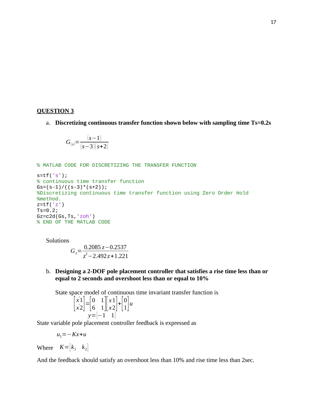
a. Discretizing continuous transfer function shown below with sampling time Ts=0.2s
G(s)= ( s−1 )
( s−3 ) ( s+2 )
% MATLAB CODE FOR DISCRETIZING THE TRANSFER FUNCTION
s=tf('s');
% continuous time transfer function
Gs=(s-1)/((s-3)*(s+2));
%Discretizing continuous time transfer function using Zero Order Hold
%method.
z=tf('z')
Ts=0.2;
Gz=c2d(Gs,Ts,'zoh')
% END OF THE MATLAB CODE
Solutions
Gz= 0.2085 z−0.2537
z2 −2.492 z +1.221
b. Designing a 2-DOF pole placement controller that satisfies a rise time less than or
equal to 2 seconds and overshoot less than or equal to 10%
State space model of continuous time invariant transfer function is
[ ˙x 1
˙x 2 ]=[0 1
6 1 ][ x 1
x 2 ]+ [0
1 ]u
y= [−1 1 ]
State variable pole placement controller feedback is expressed as
u1=−Kx+u
Where K= [ k1 k2 ]
And the feedback should satisfy an overshoot less than 10% and rise time less than 2sec.
QUESTION 3
a. Discretizing continuous transfer function shown below with sampling time Ts=0.2s
G(s)= ( s−1 )
( s−3 ) ( s+2 )
% MATLAB CODE FOR DISCRETIZING THE TRANSFER FUNCTION
s=tf('s');
% continuous time transfer function
Gs=(s-1)/((s-3)*(s+2));
%Discretizing continuous time transfer function using Zero Order Hold
%method.
z=tf('z')
Ts=0.2;
Gz=c2d(Gs,Ts,'zoh')
% END OF THE MATLAB CODE
Solutions
Gz= 0.2085 z−0.2537
z2 −2.492 z +1.221
b. Designing a 2-DOF pole placement controller that satisfies a rise time less than or
equal to 2 seconds and overshoot less than or equal to 10%
State space model of continuous time invariant transfer function is
[ ˙x 1
˙x 2 ]=[0 1
6 1 ][ x 1
x 2 ]+ [0
1 ]u
y= [−1 1 ]
State variable pole placement controller feedback is expressed as
u1=−Kx+u
Where K= [ k1 k2 ]
And the feedback should satisfy an overshoot less than 10% and rise time less than 2sec.
18
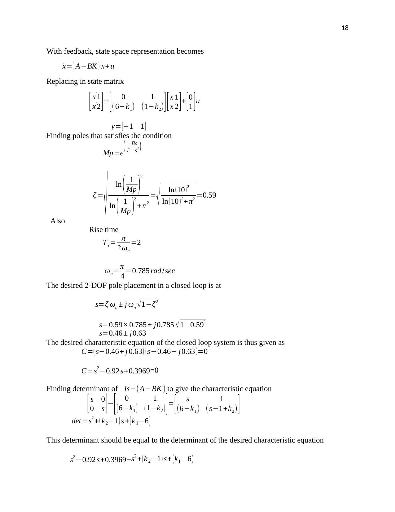
With feedback, state space representation becomes
˙x= ( A−BK ) x+ u
Replacing in state matrix
[ ˙x 1
˙x 2 ]=
[ 0 1
(6−k1) (1−k2) ] [x 1
x 2 ]+ [0
1 ]u
y= [−1 1 ]
Finding poles that satisfies the condition
Mp=e ( − Πς
√1−ς 2 )
ζ =
√ ln ( 1
Mp )2
ln ( 1
Mp )2
+ π2
= √ ln ( 10 )2
ln ( 10 )2 + π2 =0.59
Also
Rise time
T r= π
2 ωn
=2
ωn= π
4 =0.785 rad /sec
The desired 2-DOF pole placement in a closed loop is at
s=ζ ωn ± j ωn √ 1−ζ2
s=0.59× 0.785 ± j0.785 √ 1−0.592
s=0.46 ± j0.63
The desired characteristic equation of the closed loop system is thus given as
C= ( s−0.46+ j 0.63 ) ( s−0.46− j 0.63 )=0
C=s2−0.92 s+0.3969=0
Finding determinant of Is−( A−BK ) to give the characteristic equation
[ s 0
0 s ]− [ 0 1
( 6−k1 ) ( 1−k2 ) ]= [ s 1
(6−k1 ) (s−1+k2 ) ]
det =s2 + ( k2−1 ) s + ( k 1−6 )
This determinant should be equal to the determinant of the desired characteristic equation
s2−0.92 s+0.3969=s2 + (k 2−1 ) s+ ( k1−6 )
19
Solving for unknown values
( k 2−1 )=−0.92→ k2=0.08
( k 1−6 ) =0.3969 → k1=6.3969
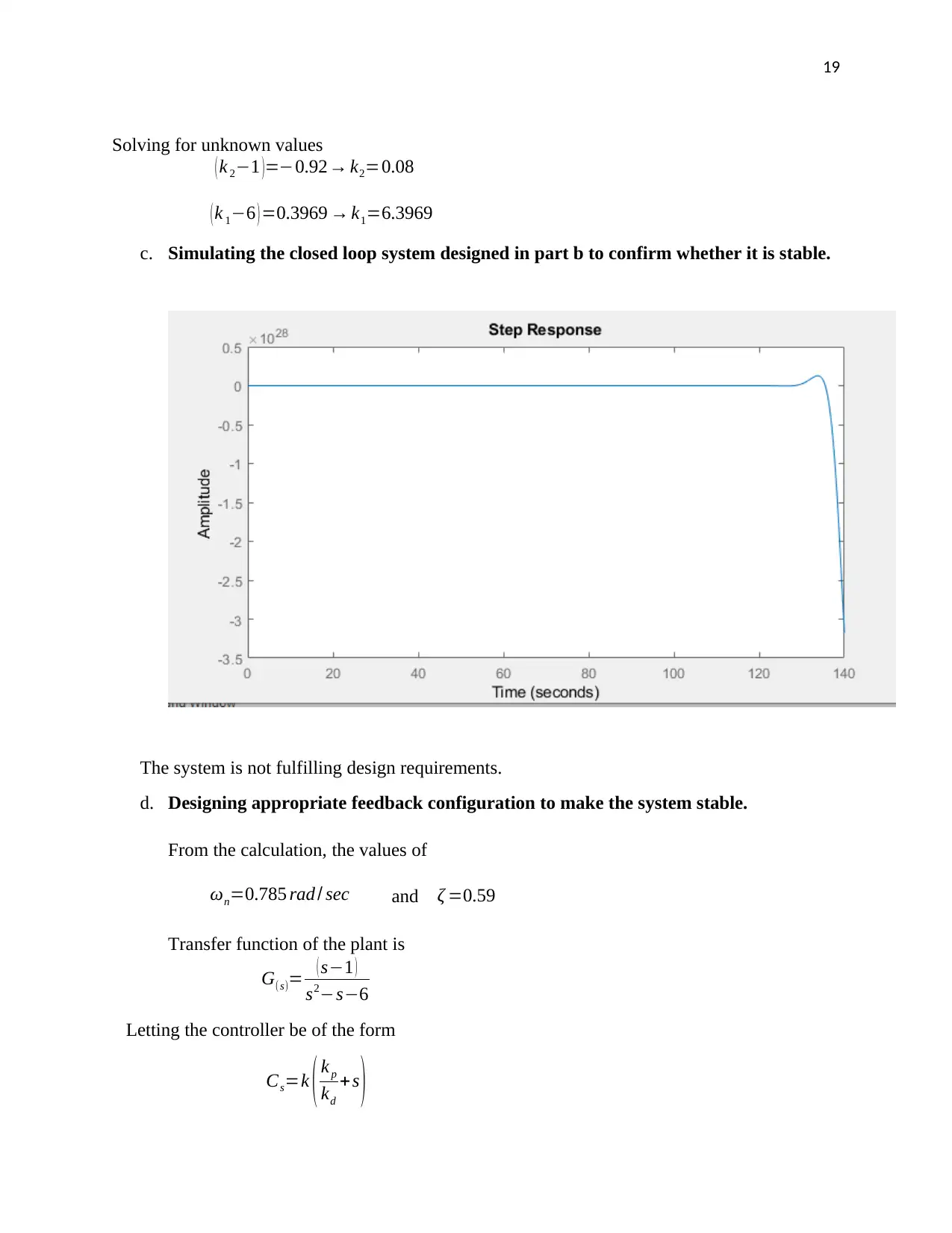
c. Simulating the closed loop system designed in part b to confirm whether it is stable.
The system is not fulfilling design requirements.
d. Designing appropriate feedback configuration to make the system stable.
From the calculation, the values of
ωn=0.785 rad / sec and ζ =0.59
Transfer function of the plant is
G(s)= ( s−1 )
s2−s−6
Letting the controller be of the form
Cs=k ( k p
kd
+s )
Solving for unknown values
( k 2−1 )=−0.92→ k2=0.08
( k 1−6 ) =0.3969 → k1=6.3969
c. Simulating the closed loop system designed in part b to confirm whether it is stable.
The system is not fulfilling design requirements.
d. Designing appropriate feedback configuration to make the system stable.
From the calculation, the values of
ωn=0.785 rad / sec and ζ =0.59
Transfer function of the plant is
G(s)= ( s−1 )
s2−s−6
Letting the controller be of the form
Cs=k ( k p
kd
+s )
Paraphrase This Document
Need a fresh take? Get an instant paraphrase of this document with our AI Paraphraser
20
The zero of the controller
z= k p
k d
The characteristic equation of the closed loop
1+Cs G(s)=1+ k (s+z ) ( s−1 )
s2−s−6
1+Cs G(s)=s2 ( k−1 ) +s ( z−2 )− ( 6+kz )=0
¿ s2 + s (z−2)
( k−1 ) − ( 6+kz )
( k −1 ) =0
But for second degree transfer function, the characteristic equation is
C=s2 + ( 2 ζ ωn ) s+ ( ωn )2 =0
Therefore
( z−2)
( k −1 ) = ( 2 ζ ωn ) =2 ×0.785 ×0.59=0.9263
z−0.9263 k =1.0737 (a)
Also
( 6+kz )
( k−1 ) = ( ωn )2=0.7852=0.6162
k ( z−0.6162 ) =−6.6162 (b)
Solving equation (a) and (b) simultaneously
z=−14.02∧k=0.4520
Following matlab code computes controller transfer function, closed loop transfer function and
then plots step response of the closed loop
clc
clear all
% matlab code computes controller transfer function,
%--closed loop transfer function and then plots step
%--response of the closed loop
%---------------------------------------------
%Transfer function
Gs=tf([1 -1],[1 -1 -6]);
%Zero of the controller
z=-14.02;
21
%Gain of the controller
k=0.4520;
%Transfer fucntion of the controller
C=tf(k*[1 z],[1])
%Closed loop transfer function of the system
G_cl=feedback(C*Gs,1)
step(G_cl)
stepinfo(G_cl)
%---------------------------------------------------------------
Controller transfer function by replacing values of (z and k) becomes
Cs=0.452 s−6.337
Closed loop transfer function of the system is
Gcl = 0.452 s2−6.789 s+6.337
1.452 s2−7.789 s+0.337
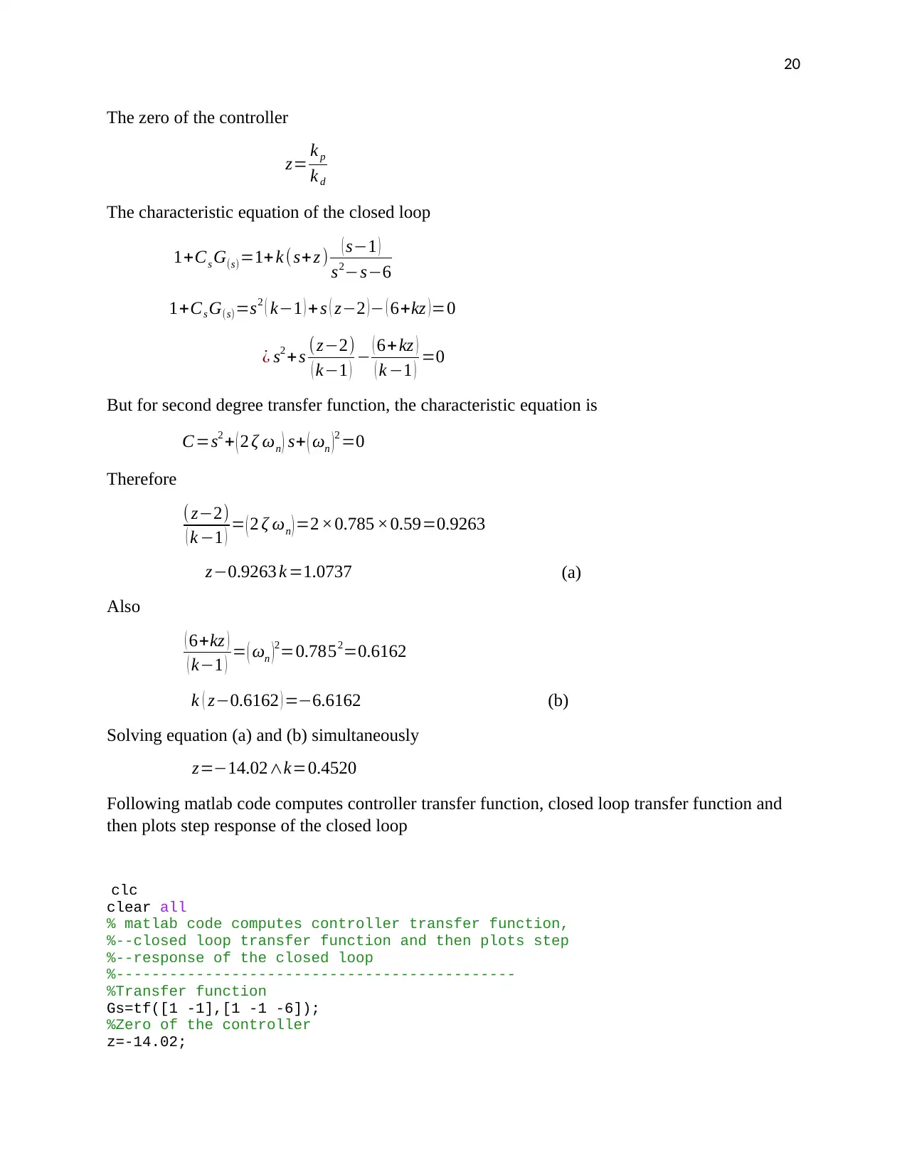
The closed loop transfer function has got same number of poles and zeros;
The step response of feedback is as shown below
The system is still unstable and does not satisfy the conditions
SISOTOOL controller tuning is therefore invoked in matlab and the controller designed
%Gain of the controller
k=0.4520;
%Transfer fucntion of the controller
C=tf(k*[1 z],[1])
%Closed loop transfer function of the system
G_cl=feedback(C*Gs,1)
step(G_cl)
stepinfo(G_cl)
%---------------------------------------------------------------
Controller transfer function by replacing values of (z and k) becomes
Cs=0.452 s−6.337
Closed loop transfer function of the system is
Gcl = 0.452 s2−6.789 s+6.337
1.452 s2−7.789 s+0.337
The closed loop transfer function has got same number of poles and zeros;
The step response of feedback is as shown below
The system is still unstable and does not satisfy the conditions
SISOTOOL controller tuning is therefore invoked in matlab and the controller designed
22
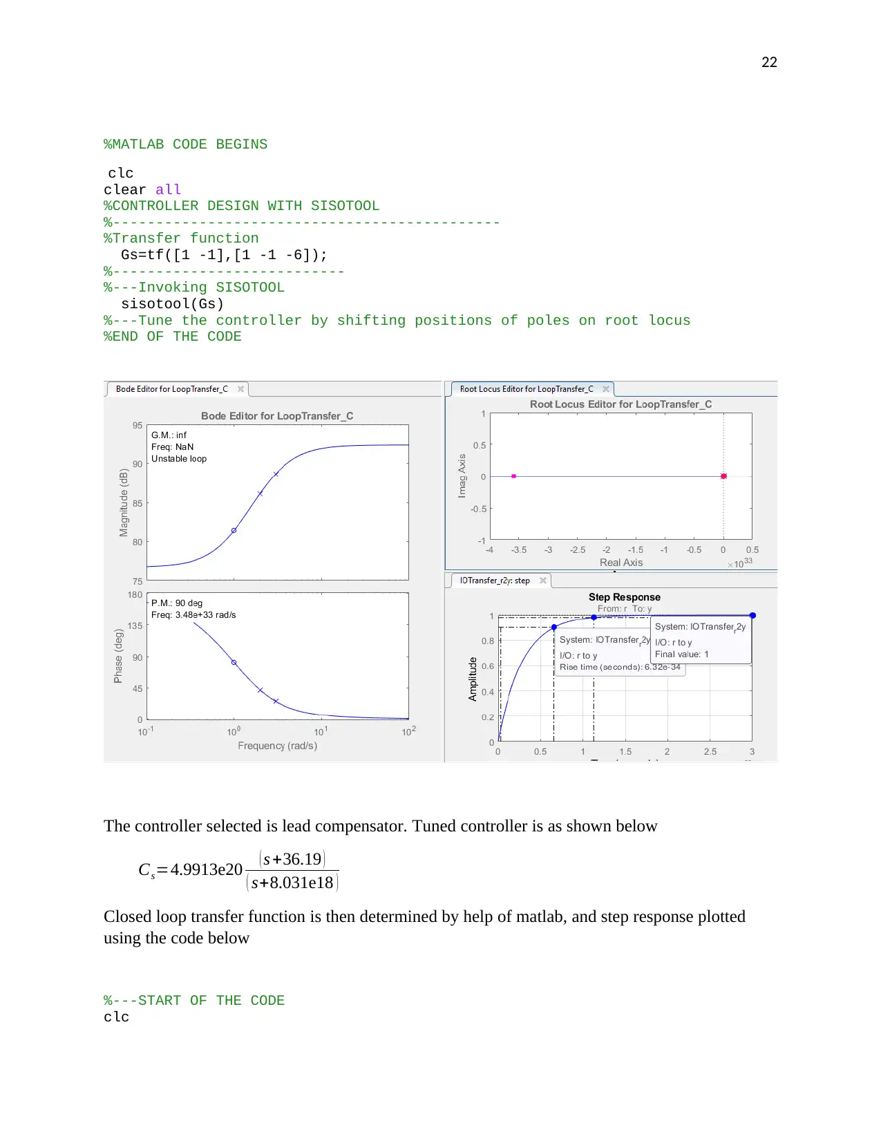
%MATLAB CODE BEGINS
clc
clear all
%CONTROLLER DESIGN WITH SISOTOOL
%---------------------------------------------
%Transfer function
Gs=tf([1 -1],[1 -1 -6]);
%---------------------------
%---Invoking SISOTOOL
sisotool(Gs)
%---Tune the controller by shifting positions of poles on root locus
%END OF THE CODE
The controller selected is lead compensator. Tuned controller is as shown below
Cs=4.9913e20 ( s +36.19 )
( s+8.031e18 )
Closed loop transfer function is then determined by help of matlab, and step response plotted
using the code below
%---START OF THE CODE
clc
Secure Best Marks with AI Grader
Need help grading? Try our AI Grader for instant feedback on your assignments.
23
clear all
%CONTROLLER DESIGN WITH SISOTOOL
%---------------------------------------------
%Transfer function
Gs=tf([1 -1],[1 -1 -6]);
%---------------------------
%---Designed controller by SISOTOOL
Cs=tf(4.9913e20*[1 36.19],[1 1.157e12]);
%--Transfer function of the closed loop
G_cl=feedback(Cs*Gs,1);
%---Plotting step response of the closed loop
step(G_cl)
stepinfo(G_cl)
%----END OF THE CODE-------------------------------
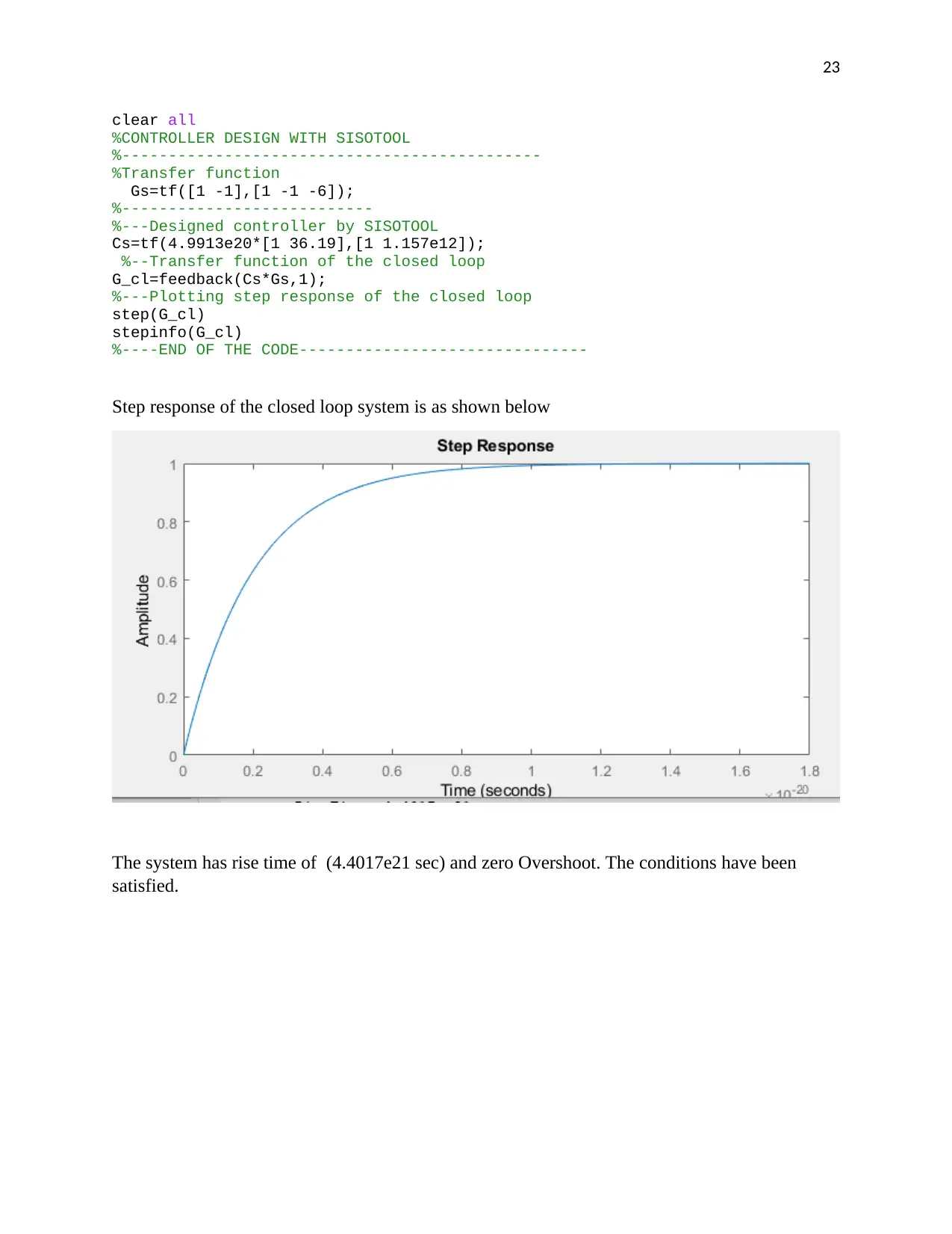
Step response of the closed loop system is as shown below
The system has rise time of (4.4017e21 sec) and zero Overshoot. The conditions have been
satisfied.
clear all
%CONTROLLER DESIGN WITH SISOTOOL
%---------------------------------------------
%Transfer function
Gs=tf([1 -1],[1 -1 -6]);
%---------------------------
%---Designed controller by SISOTOOL
Cs=tf(4.9913e20*[1 36.19],[1 1.157e12]);
%--Transfer function of the closed loop
G_cl=feedback(Cs*Gs,1);
%---Plotting step response of the closed loop
step(G_cl)
stepinfo(G_cl)
%----END OF THE CODE-------------------------------
Step response of the closed loop system is as shown below
The system has rise time of (4.4017e21 sec) and zero Overshoot. The conditions have been
satisfied.
24
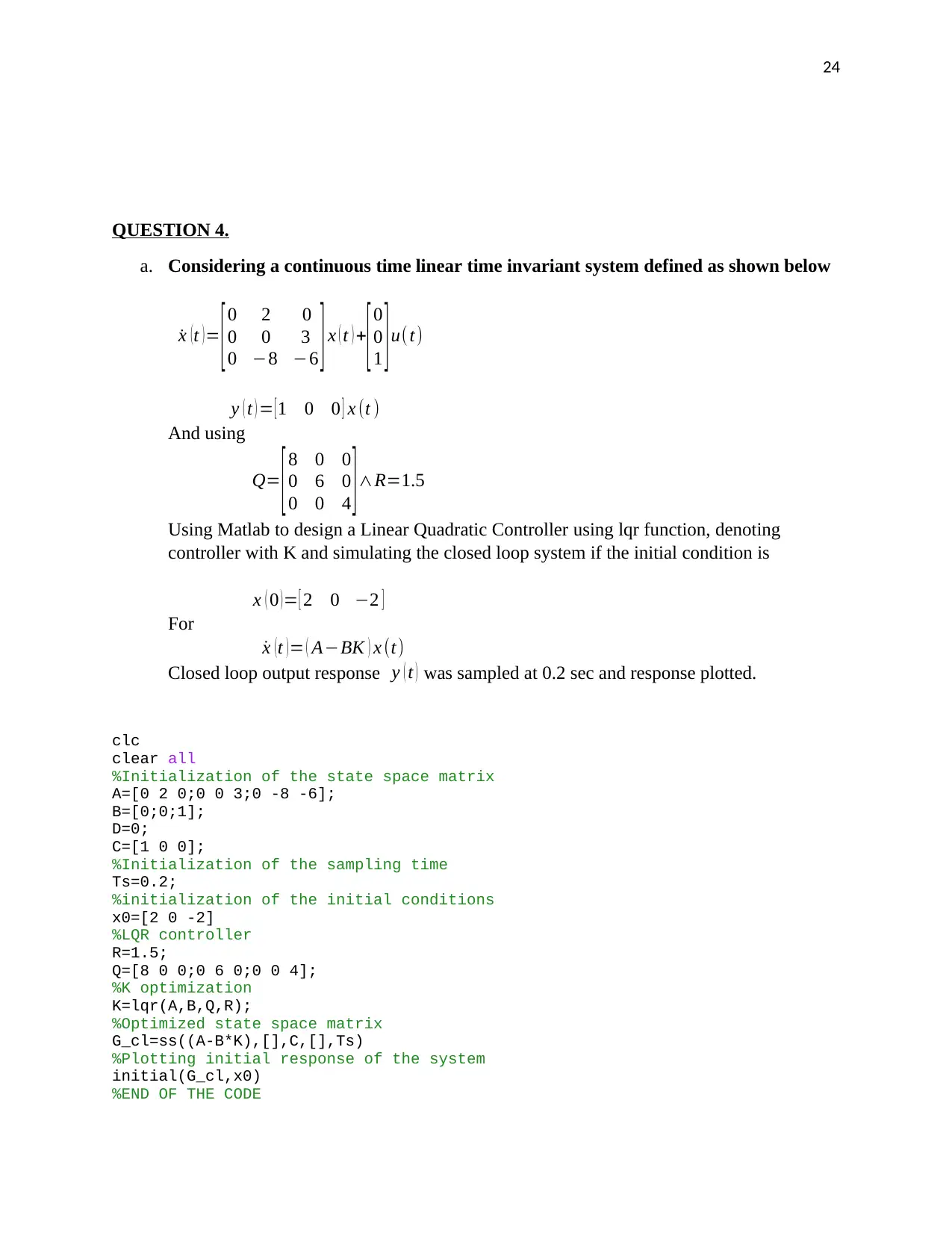
QUESTION 4.
a. Considering a continuous time linear time invariant system defined as shown below
˙x (t )= [0 2 0
0 0 3
0 −8 −6 ] x ( t ) +
[0
0
1 ]u( t)
y ( t ) = [ 1 0 0 ] x (t )
And using
Q= [ 8 0 0
0 6 0
0 0 4 ] ∧R=1.5
Using Matlab to design a Linear Quadratic Controller using lqr function, denoting
controller with K and simulating the closed loop system if the initial condition is
x ( 0 )= [ 2 0 −2 ]
For
˙x ( t ) = ( A−BK ) x (t)
Closed loop output response y ( t ) was sampled at 0.2 sec and response plotted.
clc
clear all
%Initialization of the state space matrix
A=[0 2 0;0 0 3;0 -8 -6];
B=[0;0;1];
D=0;
C=[1 0 0];
%Initialization of the sampling time
Ts=0.2;
%initialization of the initial conditions
x0=[2 0 -2]
%LQR controller
R=1.5;
Q=[8 0 0;0 6 0;0 0 4];
%K optimization
K=lqr(A,B,Q,R);
%Optimized state space matrix
G_cl=ss((A-B*K),[],C,[],Ts)
%Plotting initial response of the system
initial(G_cl,x0)
%END OF THE CODE
25
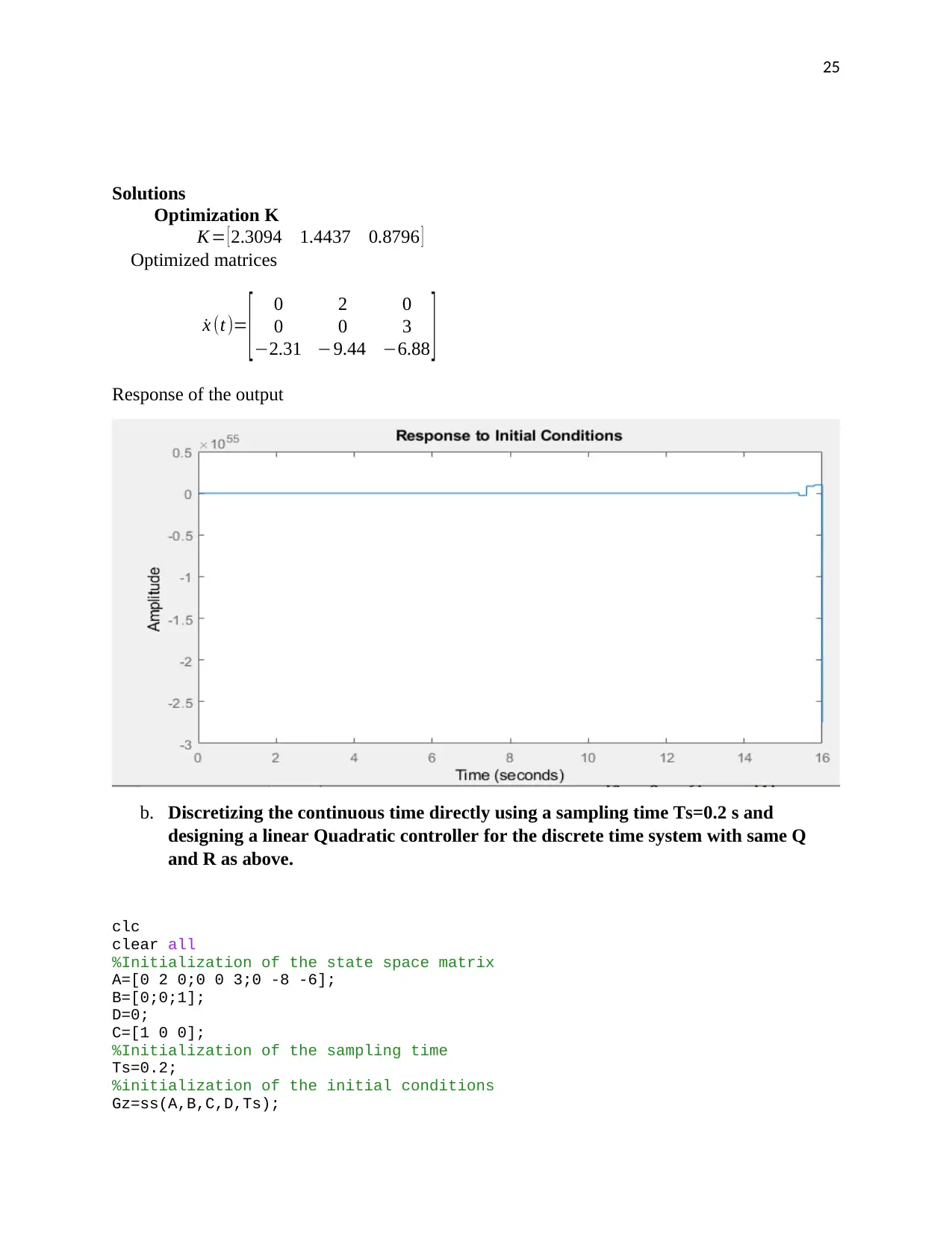
Solutions
Optimization K
K= [ 2.3094 1.4437 0.8796 ]
Optimized matrices
˙x (t)= [ 0 2 0
0 0 3
−2.31 −9.44 −6.88 ]
Response of the output
b. Discretizing the continuous time directly using a sampling time Ts=0.2 s and
designing a linear Quadratic controller for the discrete time system with same Q
and R as above.
clc
clear all
%Initialization of the state space matrix
A=[0 2 0;0 0 3;0 -8 -6];
B=[0;0;1];
D=0;
C=[1 0 0];
%Initialization of the sampling time
Ts=0.2;
%initialization of the initial conditions
Gz=ss(A,B,C,D,Ts);
Paraphrase This Document
Need a fresh take? Get an instant paraphrase of this document with our AI Paraphraser
26
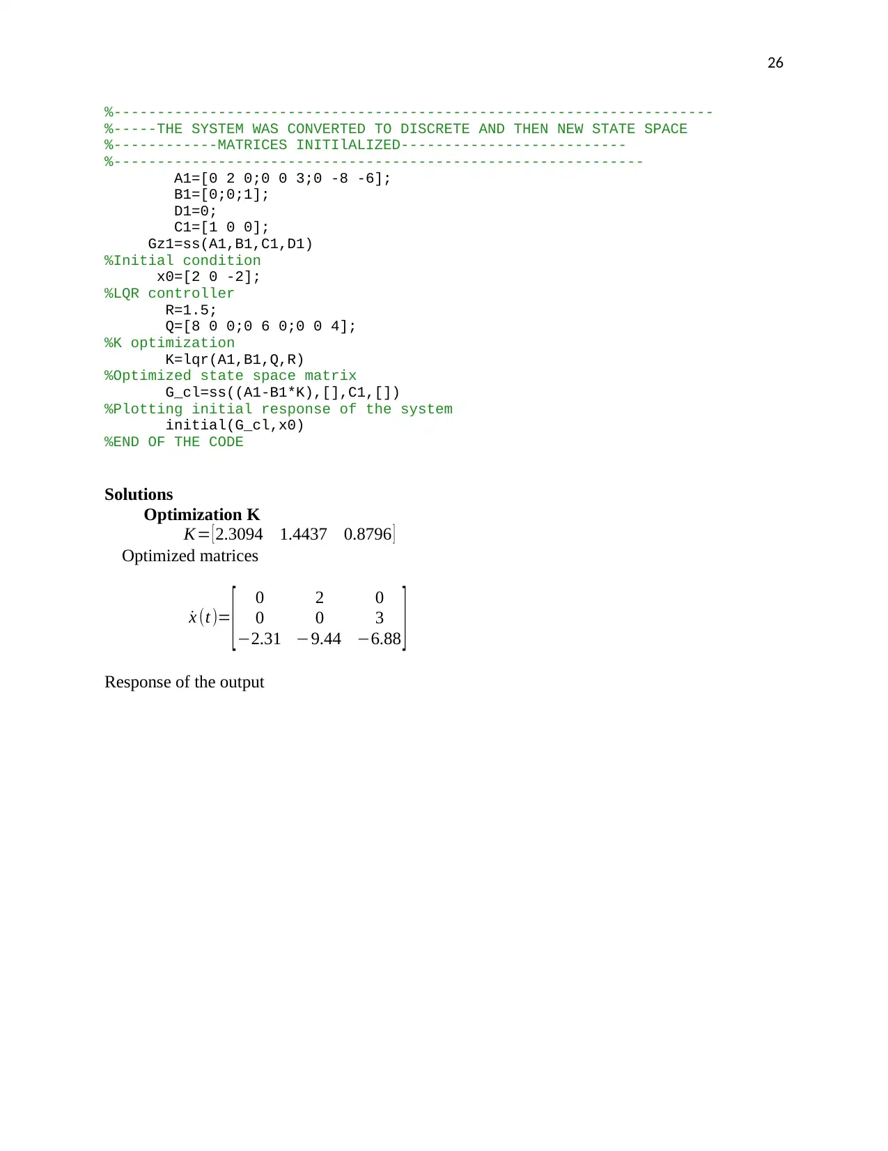
%---------------------------------------------------------------------
%-----THE SYSTEM WAS CONVERTED TO DISCRETE AND THEN NEW STATE SPACE
%------------MATRICES INITIlALIZED--------------------------
%-------------------------------------------------------------
A1=[0 2 0;0 0 3;0 -8 -6];
B1=[0;0;1];
D1=0;
C1=[1 0 0];
Gz1=ss(A1,B1,C1,D1)
%Initial condition
x0=[2 0 -2];
%LQR controller
R=1.5;
Q=[8 0 0;0 6 0;0 0 4];
%K optimization
K=lqr(A1,B1,Q,R)
%Optimized state space matrix
G_cl=ss((A1-B1*K),[],C1,[])
%Plotting initial response of the system
initial(G_cl,x0)
%END OF THE CODE
Solutions
Optimization K
K= [ 2.3094 1.4437 0.8796 ]
Optimized matrices
˙x (t)= [ 0 2 0
0 0 3
−2.31 −9.44 −6.88 ]
Response of the output
27
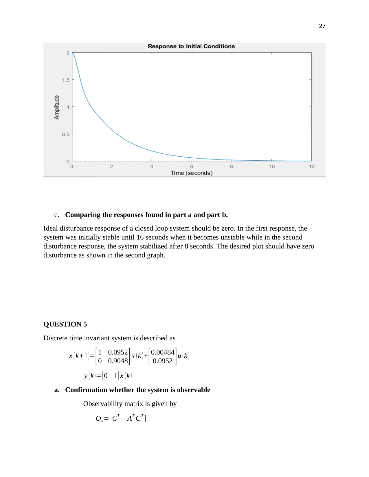
c. Comparing the responses found in part a and part b.
Ideal disturbance response of a closed loop system should be zero. In the first response, the
system was initially stable until 16 seconds when it becomes unstable while in the second
disturbance response, the system stabilized after 8 seconds. The desired plot should have zero
disturbance as shown in the second graph.
QUESTION 5
Discrete time invariant system is described as
x ( k +1 )= [1 0.0952
0 0.9048 ] x ( k ) + [0.00484
0.0952 ]u ( k )
y ( k )= [ 0 1 ] x ( k )
a. Confirmation whether the system is observable
Observability matrix is given by
Ob=[CT AT CT ]
28
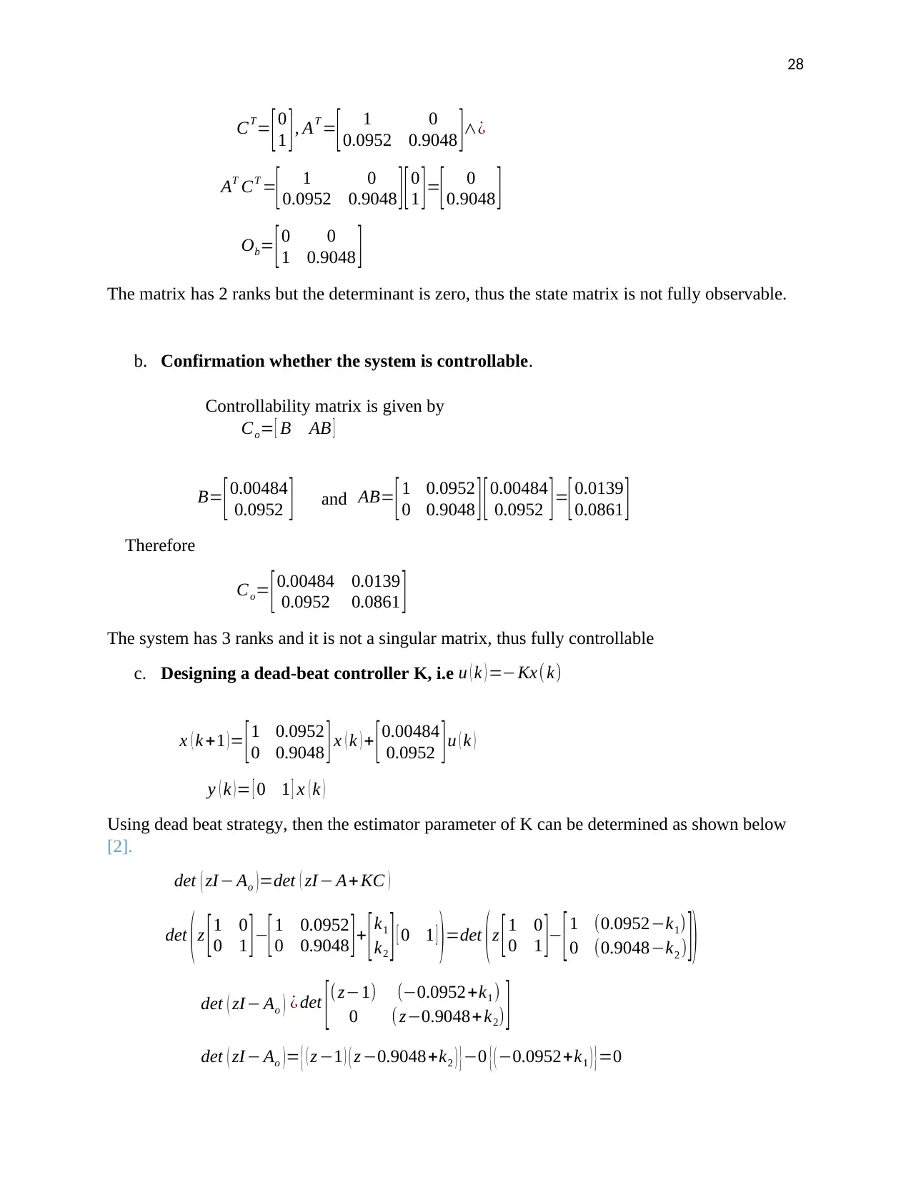
CT= [0
1 ], AT =
[ 1 0
0.0952 0.9048 ]∧¿
AT CT =
[ 1 0
0.0952 0.9048 ][ 0
1 ] =
[ 0
0.9048 ]
Ob= [0 0
1 0.9048 ]
The matrix has 2 ranks but the determinant is zero, thus the state matrix is not fully observable.
b. Confirmation whether the system is controllable.
Controllability matrix is given by
Co= [ B AB ]
B= [0.00484
0.0952 ] and AB= [ 1 0.0952
0 0.9048 ][ 0.00484
0.0952 ] =
[ 0.0139
0.0861 ]
Therefore
Co= [ 0.00484 0.0139
0.0952 0.0861 ]
The system has 3 ranks and it is not a singular matrix, thus fully controllable
c. Designing a dead-beat controller K, i.e u ( k ) =−Kx( k)
x ( k +1 ) = [ 1 0.0952
0 0.9048 ] x ( k ) + [ 0.00484
0.0952 ] u ( k )
y ( k )= [ 0 1 ] x ( k )
Using dead beat strategy, then the estimator parameter of K can be determined as shown below
[2].
det ( zI− Ao ) =det ( zI− A+ KC )
det ( z [ 1 0
0 1 ] −[ 1 0.0952
0 0.9048 ] + [ k1
k2 ] [ 0 1 ] ) =det ( z [ 1 0
0 1 ]− [ 1 (0.0952−k1)
0 (0.9048−k2 ) ])
det ( zI− Ao ) ¿ det [ (z−1) (−0.0952+k1 )
0 ( z−0.9048+k2) ]
det ( zI− Ao )= { ( z −1 ) ( z −0.9048+k2 ) } −0 { ( −0.0952+k1 ) } =0
Secure Best Marks with AI Grader
Need help grading? Try our AI Grader for instant feedback on your assignments.
29
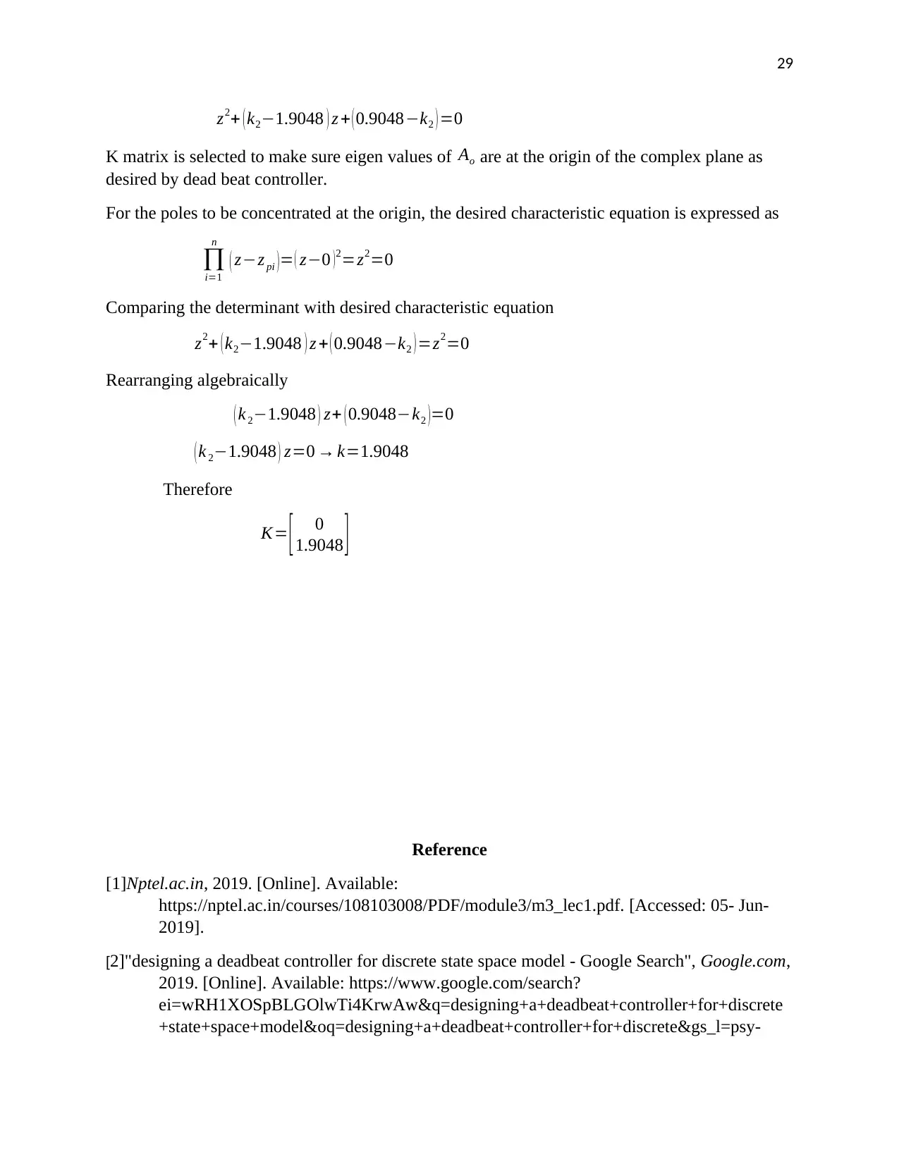
z2+ ( k2−1.9048 ) z + ( 0.9048−k2 ) =0
K matrix is selected to make sure eigen values of Ao are at the origin of the complex plane as
desired by dead beat controller.
For the poles to be concentrated at the origin, the desired characteristic equation is expressed as
∏
i=1
n
( z−z pi )= ( z−0 )2=z2=0
Comparing the determinant with desired characteristic equation
z2+ ( k2−1.9048 ) z + ( 0.9048−k2 ) =z2=0
Rearranging algebraically
( k 2−1.9048 ) z+ ( 0.9048−k2 )=0
( k 2−1.9048 ) z=0 → k=1.9048
Therefore
K= [ 0
1.9048 ]
Reference
[1]Nptel.ac.in, 2019. [Online]. Available:
https://nptel.ac.in/courses/108103008/PDF/module3/m3_lec1.pdf. [Accessed: 05- Jun-
2019].
[2]"designing a deadbeat controller for discrete state space model - Google Search", Google.com,
2019. [Online]. Available: https://www.google.com/search?
ei=wRH1XOSpBLGOlwTi4KrwAw&q=designing+a+deadbeat+controller+for+discrete
+state+space+model&oq=designing+a+deadbeat+controller+for+discrete&gs_l=psy-

30
ab.1.0.35i39.1471386.1472372..1478357...0.0..1.259.1225.2-5......0....1..gws-
wiz.......0i71.mrIBNfI9kZk. [Accessed: 05- Jun- 2019].
ab.1.0.35i39.1471386.1472372..1478357...0.0..1.259.1225.2-5......0....1..gws-
wiz.......0i71.mrIBNfI9kZk. [Accessed: 05- Jun- 2019].
1 out of 30
Related Documents


Your All-in-One AI-Powered Toolkit for Academic Success.
+13062052269
info@desklib.com
Available 24*7 on WhatsApp / Email
![[object Object]](/_next/static/media/star-bottom.7253800d.svg)
Unlock your academic potential
© 2024 | Zucol Services PVT LTD | All rights reserved.