Understanding the Scientific Method
VerifiedAdded on 2023/01/18
|15
|4090
|60
AI Summary
This article explains the scientific method and its steps for experimentation and discovery. It discusses the importance of observations, hypotheses, experiments, and data analysis in the scientific process.
Contribute Materials
Your contribution can guide someone’s learning journey. Share your
documents today.
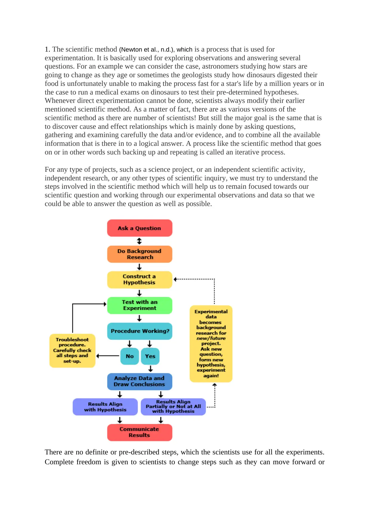
1. The scientific method (Newton et al., n.d.), which is a process that is used for
experimentation. It is basically used for exploring observations and answering several
questions. For an example we can consider the case, astronomers studying how stars are
going to change as they age or sometimes the geologists study how dinosaurs digested their
food is unfortunately unable to making the process fast for a star's life by a million years or in
the case to run a medical exams on dinosaurs to test their pre-determined hypotheses.
Whenever direct experimentation cannot be done, scientists always modify their earlier
mentioned scientific method. As a matter of fact, there are as various versions of the
scientific method as there are number of scientists! But still the major goal is the same that is
to discover cause and effect relationships which is mainly done by asking questions,
gathering and examining carefully the data and/or evidence, and to combine all the available
information that is there in to a logical answer. A process like the scientific method that goes
on or in other words such backing up and repeating is called an iterative process.
For any type of projects, such as a science project, or an independent scientific activity,
independent research, or any other types of scientific inquiry, we must try to understand the
steps involved in the scientific method which will help us to remain focused towards our
scientific question and working through our experimental observations and data so that we
could be able to answer the question as well as possible.
There are no definite or pre-described steps, which the scientists use for all the experiments.
Complete freedom is given to scientists to change steps such as they can move forward or
Secure Best Marks with AI Grader
Need help grading? Try our AI Grader for instant feedback on your assignments.
backward or can change directions. But still a good scientific investigation has got certain
features. Every investigation always begins with an observation.
• Observation – It is nothing but the use of senses to study something. Several tools such as a
microscope or a scale are used by the scientists to observe. A question follows the
observations.
• Researching – It refers to reading the already available literatures to gather information for
that subject.
• Hypothesizing – It is one of the possible explanations for an observation.
• Designing an experiment – experimentation supports or rejects your hypothesis
• (Variables) – These are the values that can change during the course of any experiment.
These affect the outcome or course of any experiment. Each experiment must contain a
dependent and an independent variable.
• Collection, organization, and analysis of data
• Reporting the results so that other scientists may test your conclusions
Q-2.
Multiple Regression (Davison, 2003) is an extension of simple linear regression.
y=¿
where∈=error term .
Two or more independent variables (Dependent variables) Multiple
regression(many to- one).
As we go on adding more and more independent variables to a multiple regression
procedure, it does not mean the regression will be better or offers better predictions.
As a matter of fact it can make things worse. This is called over fitting
As we go adding more independent variables, it creates more relationships among
them. So we can say that the independent variables are not only potentially dependent
on the dependent variables, but they are also potentially related to each other. This
situation highly should be avoided. It is called multicollinearity.
The ideal situation should be that all the independent variables are to be correlated
with the dependent variables but not with each other.
Because of these factors such as multicollinearity and overfitting, we are having a fair
amount of prep-work to be done before conducting multiple regression analysis if one
has to do it properly.
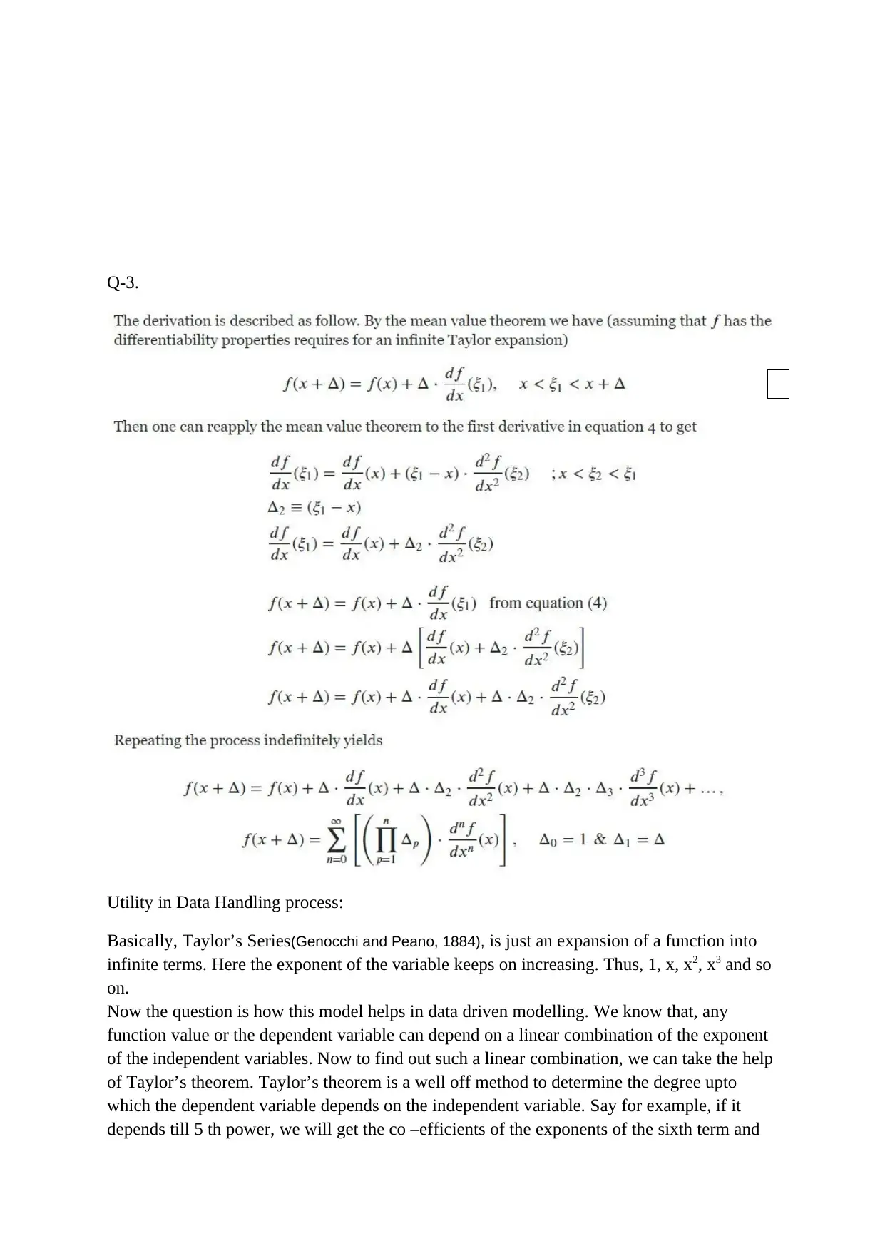
Q-3.
Utility in Data Handling process:
Basically, Taylor’s Series(Genocchi and Peano, 1884), is just an expansion of a function into
infinite terms. Here the exponent of the variable keeps on increasing. Thus, 1, x, x2, x3 and so
on.
Now the question is how this model helps in data driven modelling. We know that, any
function value or the dependent variable can depend on a linear combination of the exponent
of the independent variables. Now to find out such a linear combination, we can take the help
of Taylor’s theorem. Taylor’s theorem is a well off method to determine the degree upto
which the dependent variable depends on the independent variable. Say for example, if it
depends till 5 th power, we will get the co –efficients of the exponents of the sixth term and
so on as zero. Likewise we can represent a function as the linear combinantion of the
exponents of the independent variable.
Explanation of the terms:
The Taylor’s theorem about a value “a”. Here the coefficient of each term is just the rth
differentiation of the function where r is the number of the term in the series.
As fas as Taylor Series is concerned, it gives us the predicted value of any function in the
forward or backward direction. After conducting the result, we may get, match it with the
calculated value from Taylor’s theorem and subsequently obtain the errors. It is a linear
method.
Q-4.
1
Mathematical Formulation:
We at the beginning are having only two people- one male & a female. They mate and at the
end of two months we get four people i,e two males and two females. These two females
again gives birth to two babies-one male and one female each. Thus at the end of four months
we get eight people, four males and four females. These four females agains gives birth to
eight people(four males and four females) Thereby producing 8+8=16, at the end of six
months.
At the end of zero months, we are having [2 ( 0/ 2)+1
]=2 people;
At the end of 2 months, we have [2 (2 /2 )+1
]=4 people;
At the end of 4 months, we have [2 ( 4/ 2)+1
]=8 people;
At the end of 6 months, we have[2 (6 / 2)+1
]=16 people.
Solution:
Secure Best Marks with AI Grader
Need help grading? Try our AI Grader for instant feedback on your assignments.
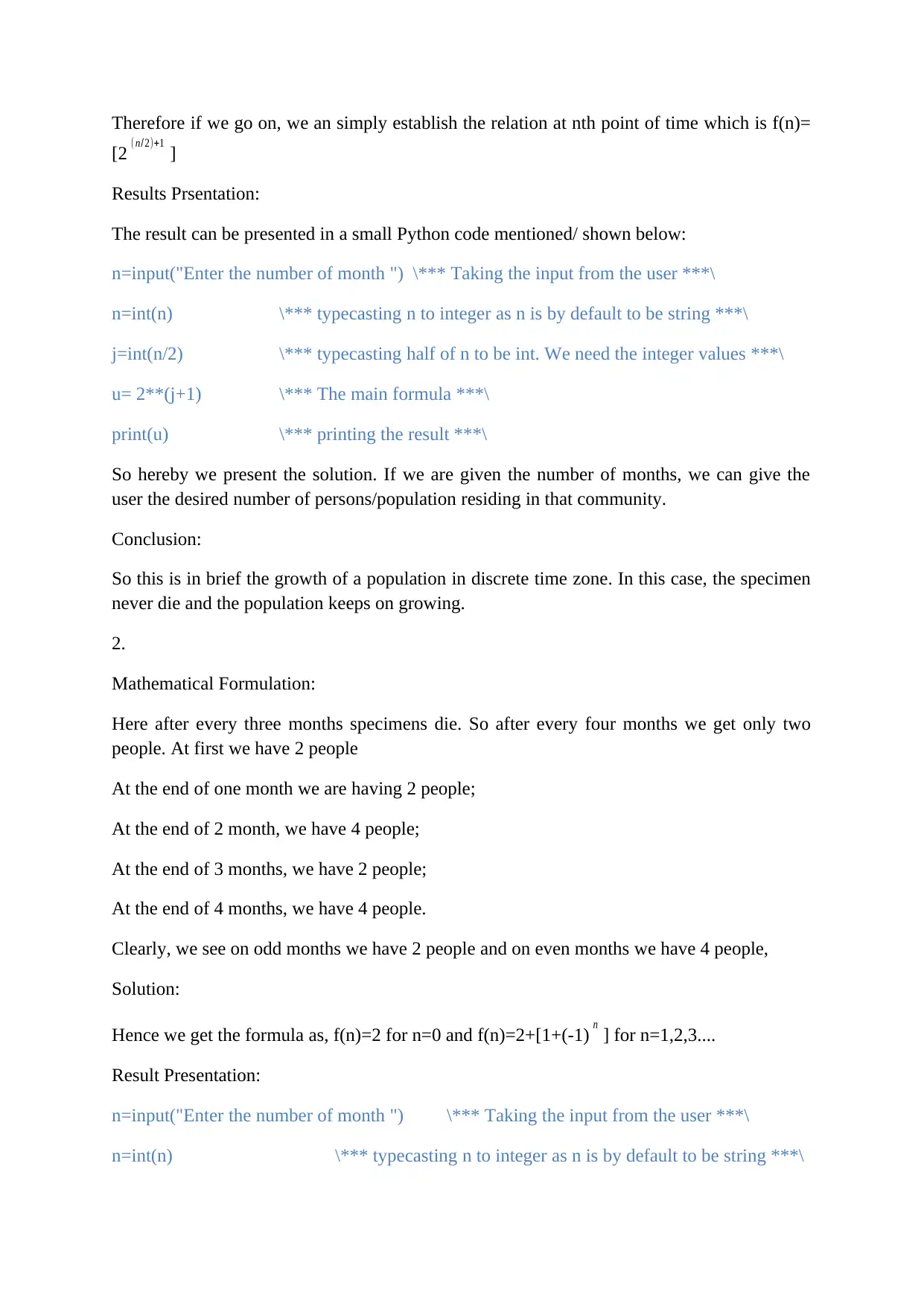
Therefore if we go on, we an simply establish the relation at nth point of time which is f(n)=
[2 ( n/ 2)+1
]
Results Prsentation:
The result can be presented in a small Python code mentioned/ shown below:
n=input("Enter the number of month ") \*** Taking the input from the user ***\
n=int(n) \*** typecasting n to integer as n is by default to be string ***\
j=int(n/2) \*** typecasting half of n to be int. We need the integer values ***\
u= 2**(j+1) \*** The main formula ***\
print(u) \*** printing the result ***\
So hereby we present the solution. If we are given the number of months, we can give the
user the desired number of persons/population residing in that community.
Conclusion:
So this is in brief the growth of a population in discrete time zone. In this case, the specimen
never die and the population keeps on growing.
2.
Mathematical Formulation:
Here after every three months specimens die. So after every four months we get only two
people. At first we have 2 people
At the end of one month we are having 2 people;
At the end of 2 month, we have 4 people;
At the end of 3 months, we have 2 people;
At the end of 4 months, we have 4 people.
Clearly, we see on odd months we have 2 people and on even months we have 4 people,
Solution:
Hence we get the formula as, f(n)=2 for n=0 and f(n)=2+[1+(-1) n
] for n=1,2,3....
Result Presentation:
n=input("Enter the number of month ") \*** Taking the input from the user ***\
n=int(n) \*** typecasting n to integer as n is by default to be string ***\
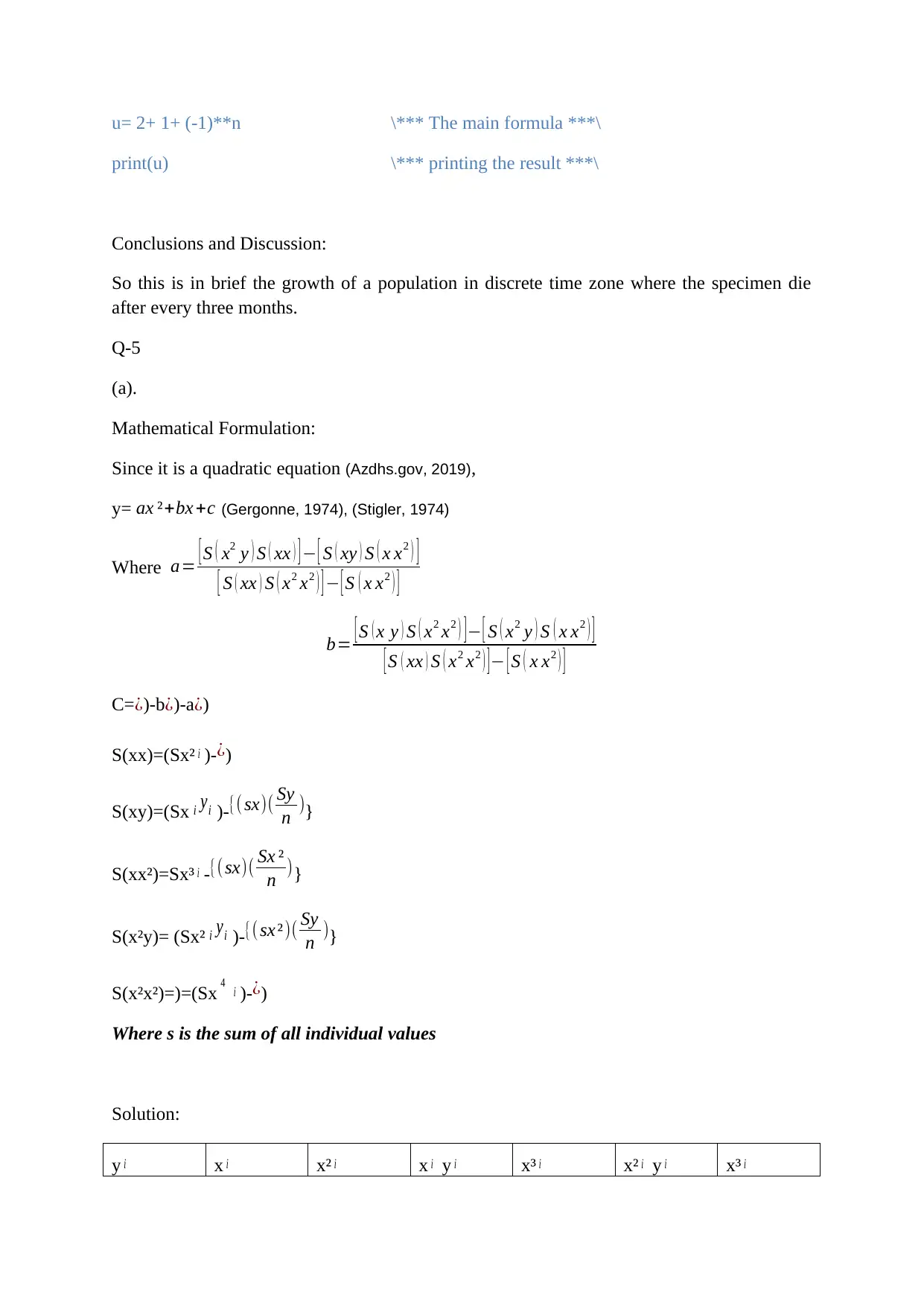
u= 2+ 1+ (-1)**n \*** The main formula ***\
print(u) \*** printing the result ***\
Conclusions and Discussion:
So this is in brief the growth of a population in discrete time zone where the specimen die
after every three months.
Q-5
(a).
Mathematical Formulation:
Since it is a quadratic equation (Azdhs.gov, 2019),
y= ax ²+bx +c (Gergonne, 1974), (Stigler, 1974)
Where a= [ S ( x2 y ) S ( xx ) ] − [ S ( xy ) S ( x x2 ) ]
[ S ( xx ) S ( x2 x2 ) ] − [ S ( x x2 ) ]
b= [ S ( x y ) S ( x2 x2 ) ] − [ S ( x2 y ) S ( x x2 ) ]
[ S ( xx ) S ( x2 x2 ) ] − [ S ( x x2 ) ]
C=¿)-b¿)-a¿)
S(xx)=(Sx² i )-¿)
S(xy)=(Sx i yi )-{( sx)( Sy
n )}
S(xx²)=Sx³ i -{(sx)( Sx ²
n )}
S(x²y)= (Sx² i yi )-{(sx ²)( Sy
n )}
S(x²x²)=)=(Sx 4 i )-¿)
Where s is the sum of all individual values
Solution:
y i x i x² i x i y i x³ i x² i y i x³ i
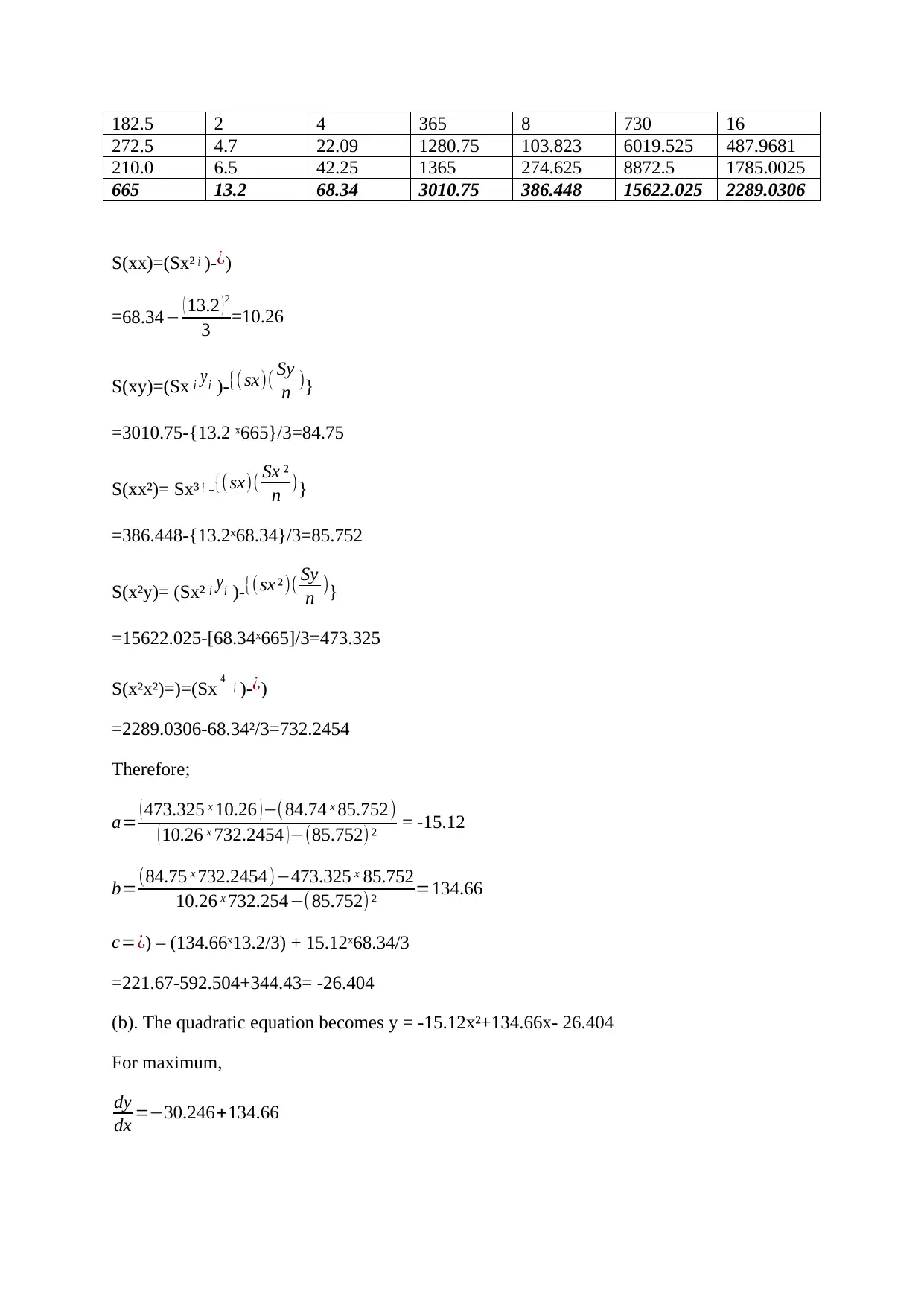
182.5 2 4 365 8 730 16
272.5 4.7 22.09 1280.75 103.823 6019.525 487.9681
210.0 6.5 42.25 1365 274.625 8872.5 1785.0025
665 13.2 68.34 3010.75 386.448 15622.025 2289.0306
S(xx)=(Sx² i )-¿)
=68.34− ( 13.2 )2
3 =10.26
S(xy)=(Sx i yi )-{( sx)( Sy
n )}
=3010.75-{13.2 ˣ665}/3=84.75
S(xx²)= Sx³ i -{(sx)( Sx ²
n )}
=386.448-{13.2ˣ68.34}/3=85.752
S(x²y)= (Sx² i yi )-{(sx ²)( Sy
n )}
=15622.025-[68.34ˣ665]/3=473.325
S(x²x²)=)=(Sx 4 i )-¿)
=2289.0306-68.34²/3=732.2454
Therefore;
a= ( 473.325 ˣ 10.26 ) −(84.74 ˣ 85.752)
( 10.26 ˣ 732.2454 ) −(85.752)² = -15.12
b=(84.75 ˣ 732.2454)−473.325 ˣ 85.752
10.26 ˣ 732.254−( 85.752)² =134.66
c=¿) – (134.66ˣ13.2/3) + 15.12ˣ68.34/3
=221.67-592.504+344.43= -26.404
(b). The quadratic equation becomes y = -15.12x²+134.66x- 26.404
For maximum,
dy
dx =−30.246+134.66
Paraphrase This Document
Need a fresh take? Get an instant paraphrase of this document with our AI Paraphraser
for maxima∨minima dy
dx =0.
⇒ -30.24x+134.66=0
⇒ x= 134.66
30.24 =4.45
Again, d ² y
dx ² = -30.24
Thus, x=4.45 is the corresponding value of x for which it is maximum.
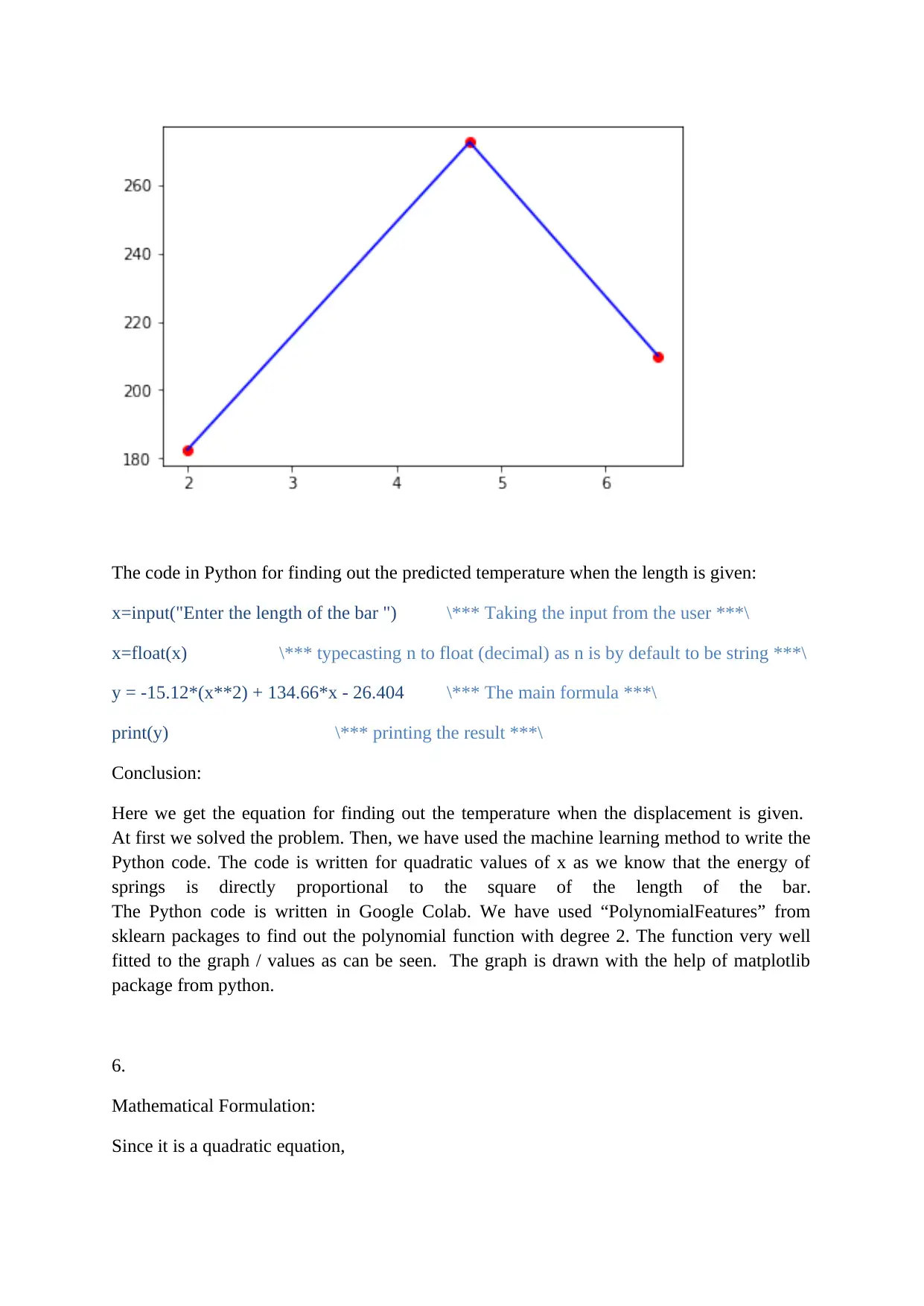
Y= -15.12ˣ4.45² +134.66ˣ4.45-26.4004 = 273.4228ºc is the max Temperature.
(c). For rightmost end of the bar, x=8
Y= -15.12ˣ64+134.66ˣ8-26.4004= -967.68+1077.28-26.4004= 83.2ºc
The experimental value is 81.5ºc
Error =1.7
Results Presentation:
From this solution, we obtain the mathematical form as shown below:
y = -15.12x²+134.66x- 26.404
Here, the variable is in quadratic form, If we draw a graph, it takes the form of a parabola.
The co-efficients of x2 , x and the constant term are -15.12, 134.66 and -26.404.
Here y is the temperature and x is the distance.
A small python code is given. Here the code applies the machine learning Polynomial
regression process to determine a good predicting function. As the number of values is very
less, there is strong doubt regarding the feasibility of the model.
\*** importing the pandas library ***\
import pandas as pd
\*** defining the list ***\
df=[[2,182.5],[4.7, 272.5],[6.5,210]]
\*** converting the list as a panda dataframe ***\
df=pd.DataFrame(df)
\*** taking only the 2D x values ***\
dx =0.
⇒ -30.24x+134.66=0
⇒ x= 134.66
30.24 =4.45
Again, d ² y
dx ² = -30.24
Thus, x=4.45 is the corresponding value of x for which it is maximum.
Y= -15.12ˣ4.45² +134.66ˣ4.45-26.4004 = 273.4228ºc is the max Temperature.
(c). For rightmost end of the bar, x=8
Y= -15.12ˣ64+134.66ˣ8-26.4004= -967.68+1077.28-26.4004= 83.2ºc
The experimental value is 81.5ºc
Error =1.7
Results Presentation:
From this solution, we obtain the mathematical form as shown below:
y = -15.12x²+134.66x- 26.404
Here, the variable is in quadratic form, If we draw a graph, it takes the form of a parabola.
The co-efficients of x2 , x and the constant term are -15.12, 134.66 and -26.404.
Here y is the temperature and x is the distance.
A small python code is given. Here the code applies the machine learning Polynomial
regression process to determine a good predicting function. As the number of values is very
less, there is strong doubt regarding the feasibility of the model.
\*** importing the pandas library ***\
import pandas as pd
\*** defining the list ***\
df=[[2,182.5],[4.7, 272.5],[6.5,210]]
\*** converting the list as a panda dataframe ***\
df=pd.DataFrame(df)
\*** taking only the 2D x values ***\
x=df.iloc[:,0:1].values
\*** taking only the y values ***\
y=df.iloc[:,1].values
\*** importing the sklearn library for polynomial operations.***\
from sklearn.preprocessing import PolynomialFeatures
\*** defining an object ‘poly’ for 2 degrees ***\
poly=PolynomialFeatures(degree=2)
\*** ‘poly_x’ takes the functionality for the data frame ‘x’ ***\
poly_x=poly.fit_transform(x)
\*** libraries imported for linear regression ***\
from sklearn.linear_model import LinearRegression
\*** regressor is an object defined from Linear Regression method ***\
regressor=LinearRegression()
\*** the functionality of regressor is defined ***\
regressor.fit(poly_x,y)
\*** matplotlib is imported for plotting ***\
import matplotlib.pyplot as plt
\*** Scatter plot is drawn ***\
plt.scatter(x,y,color='red')
\*** prediction is done ***\
plt.plot(x,regressor.predict(poly.fit_transform(x)),color='blue')
\*** plotting is done ***\
plt.show()
The code in Python for finding out the predicted temperature when the length is given:
x=input("Enter the length of the bar ") \*** Taking the input from the user ***\
x=float(x) \*** typecasting n to float (decimal) as n is by default to be string ***\
y = -15.12*(x**2) + 134.66*x - 26.404 \*** The main formula ***\
print(y) \*** printing the result ***\
Conclusion:
Here we get the equation for finding out the temperature when the displacement is given.
At first we solved the problem. Then, we have used the machine learning method to write the
Python code. The code is written for quadratic values of x as we know that the energy of
springs is directly proportional to the square of the length of the bar.
The Python code is written in Google Colab. We have used “PolynomialFeatures” from
sklearn packages to find out the polynomial function with degree 2. The function very well
fitted to the graph / values as can be seen. The graph is drawn with the help of matplotlib
package from python.
6.
Mathematical Formulation:
Since it is a quadratic equation,
Secure Best Marks with AI Grader
Need help grading? Try our AI Grader for instant feedback on your assignments.
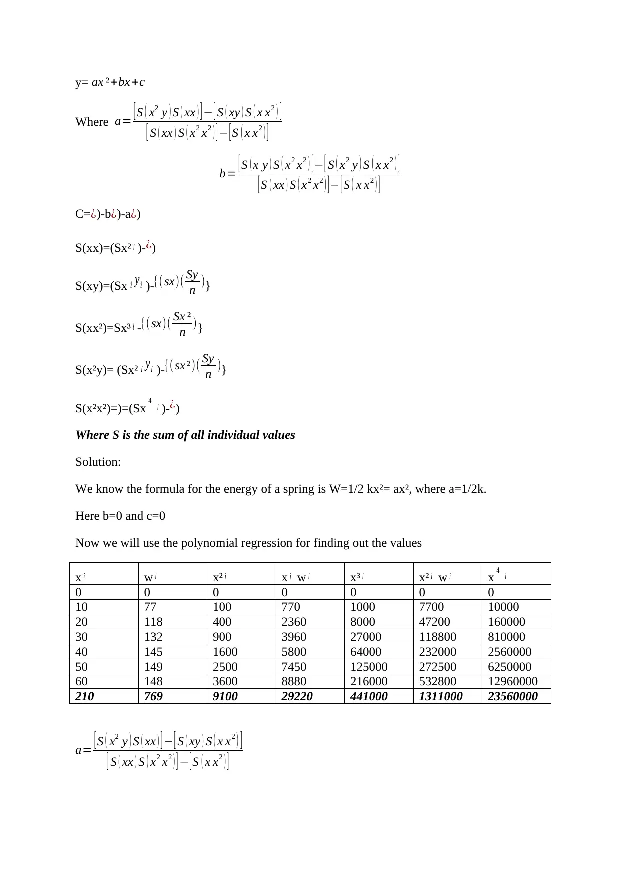
y= ax ²+bx +c
Where a= [ S ( x2 y ) S ( xx ) ] − [ S ( xy ) S ( x x2 ) ]
[ S ( xx ) S ( x2 x2 ) ] − [ S ( x x2 ) ]
b= [ S ( x y ) S ( x2 x2 ) ] − [ S ( x2 y ) S ( x x2 ) ]
[ S ( xx ) S ( x2 x2 ) ] − [ S ( x x2 ) ]
C=¿)-b¿)-a¿)
S(xx)=(Sx² i )-¿)
S(xy)=(Sx i yi )-{( sx)( Sy
n )}
S(xx²)=Sx³ i -{(sx)( Sx ²
n )}
S(x²y)= (Sx² i yi )-{(sx ²)( Sy
n )}
S(x²x²)=)=(Sx 4 i )-¿)
Where S is the sum of all individual values
Solution:
We know the formula for the energy of a spring is W=1/2 kx²= ax², where a=1/2k.
Here b=0 and c=0
Now we will use the polynomial regression for finding out the values
x i w i x² i x i w i x³ i x² i w i x 4 i
0 0 0 0 0 0 0
10 77 100 770 1000 7700 10000
20 118 400 2360 8000 47200 160000
30 132 900 3960 27000 118800 810000
40 145 1600 5800 64000 232000 2560000
50 149 2500 7450 125000 272500 6250000
60 148 3600 8880 216000 532800 12960000
210 769 9100 29220 441000 1311000 23560000
a= [ S ( x2 y ) S ( xx ) ] − [ S ( xy ) S ( x x2 ) ]
[ S ( xx ) S ( x2 x2 ) ] − [ S ( x x2 ) ]
S(xx)=(Sx² i )-¿)
=9100-6300=2800
S(xw)=(Sx i wi )-{( sx)( Sw
n )}
=29220-210ˣ769/7=6150
S(xx²)= Sx³ i -{(sx)( Sx ²
n )}
=441000-210ˣ9100/7=168000
S(x²w)= (Sx² i wi )-{( sx ²)( Sw
n )}
1311000-9100ˣ769/7= 311300
S(x²x²)=)=(Sx 4 i )-¿)
=23560000-9100²/7= 11730000
a= 311300× 2800−6150 ×168000
2800 ×11730000−168000² =−16156
4620 10= -3.5 ×10
a=1/2k, k=2a= 2×(-3.5×10)= -7 ×10N/mm²
w=1/2kx²=−7 ×10 x2
2 = -3.5 ×10 8 x2
Results Presentation:
From this solution, we obtain the mathematical form as shown below:
w=1/2kx²=−7 ×10 x2
2 = -3.5×10 8 x2
Here W is the work and x is the distance.
A small python code is given. Here the code applies the machine learning Polynomial
regression process to determine a good predicting function. As the number of values is very
less, there is strong doubt regarding the feasibility of the model.
\*** importing the pandas library ***\
import pandas as pd
\*** defining the list ***\
df=[[0,0],[10,77],[20,118],[30,132],[40,145],[50,149],[60,148]]
\*** converting the list as a panda dataframe ***\
df=pd.DataFrame(df)
\*** taking only 2D x values ***\
x=df.iloc[:,0:1].values
\*** taking only the y values ***\
y=df.iloc[:,1].values
\*** importing the sklearn library for polynomial operations.***\
from sklearn.preprocessing import PolynomialFeatures
\*** defining an object ‘poly’ for 2 degrees ***\
poly=PolynomialFeatures(degree=2)
\*** ‘poly_x’ takes the functionality for the data frame ‘x’ ***\
poly_x=poly.fit_transform(x)
\*** libraries imported for linear regression ***\
from sklearn.linear_model import LinearRegression
\*** regressor is an object defined from Linear Regression method ***\
regressor=LinearRegression()
\*** the functionality of regressor is defined ***\
regressor.fit(poly_x,y)
\*** matplotlib is imported for plotting ***\
import matplotlib.pyplot as plt
\*** Scatter plot is drawn ***\
plt.scatter(x,y,color='red')
\*** prediction is done ***\
plt.plot(x,regressor.predict(poly.fit_transform(x)),color='blue')
\*** plotting is done ***\
plt.show()
Paraphrase This Document
Need a fresh take? Get an instant paraphrase of this document with our AI Paraphraser
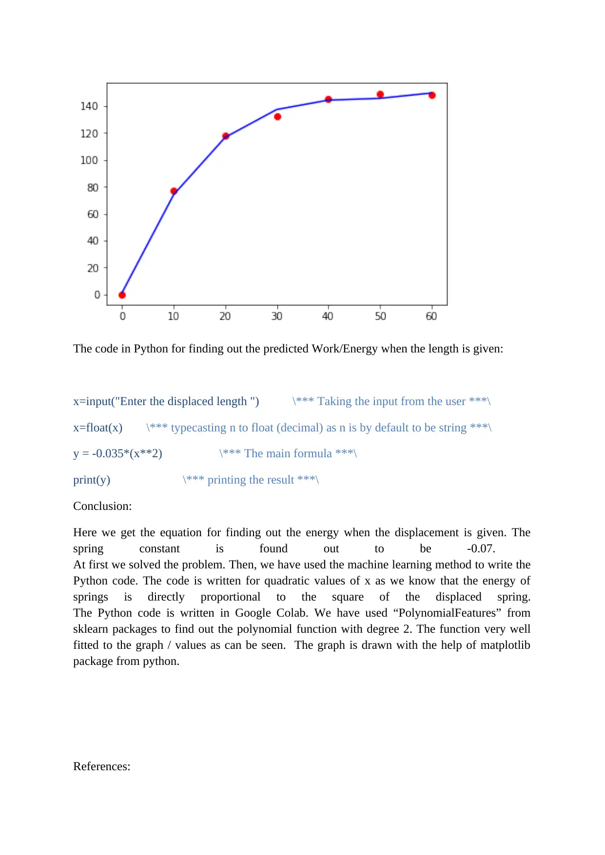
The code in Python for finding out the predicted Work/Energy when the length is given:
x=input("Enter the displaced length ") \*** Taking the input from the user ***\
x=float(x) \*** typecasting n to float (decimal) as n is by default to be string ***\
y = -0.035*(x**2) \*** The main formula ***\
print(y) \*** printing the result ***\
Conclusion:
Here we get the equation for finding out the energy when the displacement is given. The
spring constant is found out to be -0.07.
At first we solved the problem. Then, we have used the machine learning method to write the
Python code. The code is written for quadratic values of x as we know that the energy of
springs is directly proportional to the square of the displaced spring.
The Python code is written in Google Colab. We have used “PolynomialFeatures” from
sklearn packages to find out the polynomial function with degree 2. The function very well
fitted to the graph / values as can be seen. The graph is drawn with the help of matplotlib
package from python.
References:
Genocchi, A. and Peano, G. (1884). Calcolo differenziale e principii di calcolo integrale. Fratelli Bocca
ed., (67), p.XVII–XIX.
Newton, I., Budenz, J., Cohen, I. and Whitman, A. (n.d.). The Principia.
Davison, A. (2003). Statistical models. Cambridge, U.K.: Cambridge University Press.
Azdhs.gov. (2019). [online] Available at: https://www.azdhs.gov/documents/preparedness/state-
laboratory/lab-licensure-certification/technical-resources/calibration-training/12-quadratic-least-
squares-regression-calib.pdf [Accessed 23 Apr. 2019].
Gergonne, J. (1974). The application of the method of least squares to the interpolation of
sequences. Historia Mathematica, 1(4), pp.439-447.
Stigler, S. (1974). Gergonne's 1815 paper on the design and analysis of polynomial regression
experiments. Historia Mathematica, 1(4), pp.431-439.
1 out of 15
Related Documents


Your All-in-One AI-Powered Toolkit for Academic Success.
+13062052269
info@desklib.com
Available 24*7 on WhatsApp / Email
![[object Object]](/_next/static/media/star-bottom.7253800d.svg)
Unlock your academic potential
© 2024 | Zucol Services PVT LTD | All rights reserved.